can be \(\leq 1\) (the data are not guaranteed under our model)
and outside of a few special cases it is impossible to calculate in closed form
but it is extremely important because without it the posterior \(\mathbb{P}(\theta \mid \text{data})\) is not a proper probability, it could be \(> 1\)
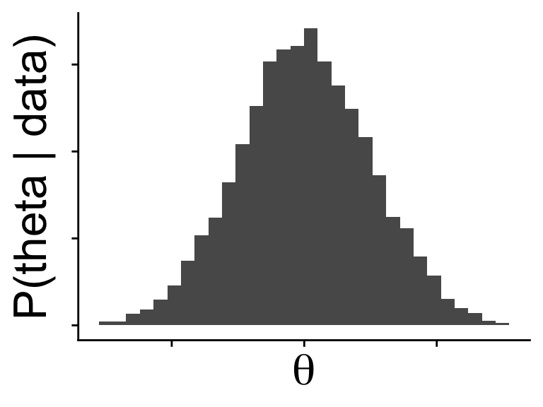
So how do we get the posterior?
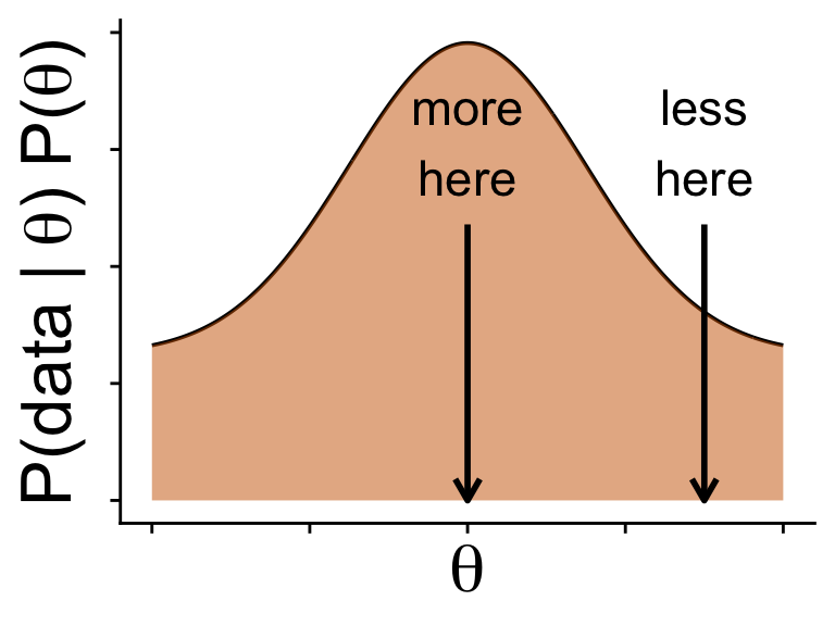
Even though we typically don’t know \(\mathbb{P}(\text{data})\) to normalize the posterior, we know the shape of the posterior
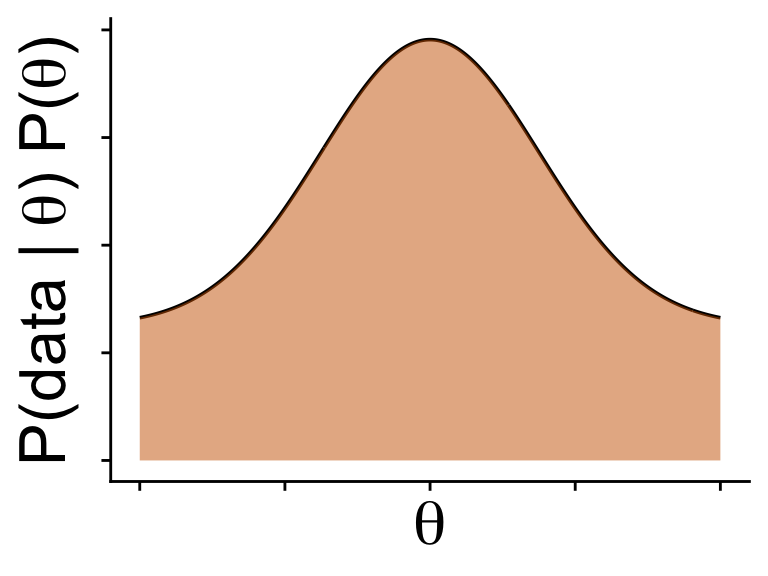
\(\mathbb{P}(\text{data} | \theta) \mathbb{P}(\theta)\) gives the shape
does not sum to 1 (not a proper probability)
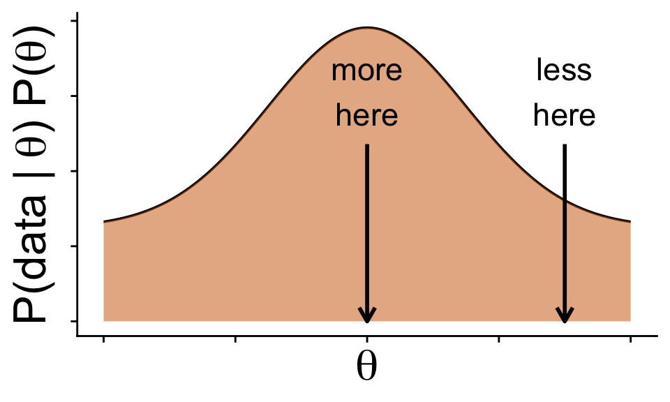
but does show regions where probability should be higher and lower
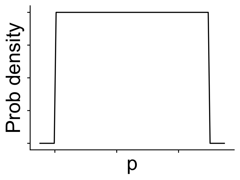
for a single value of \(\theta\) we always know \(\mathbb{P}(\text{data} | \theta)\) and \(\mathbb{P}(\theta)\)
So how do we get the posterior?
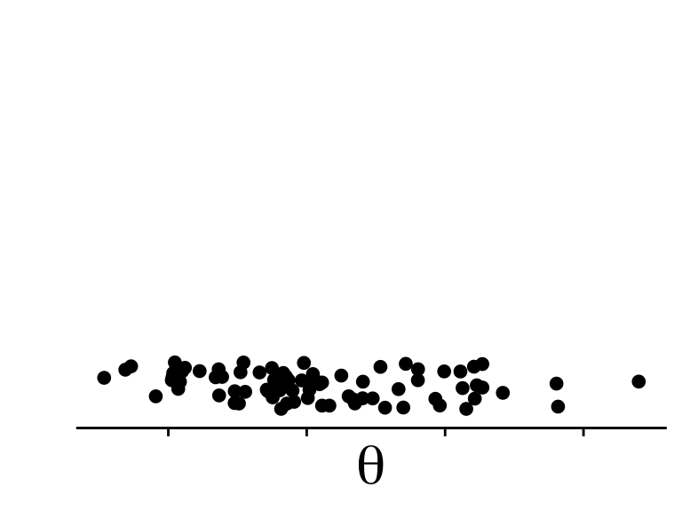
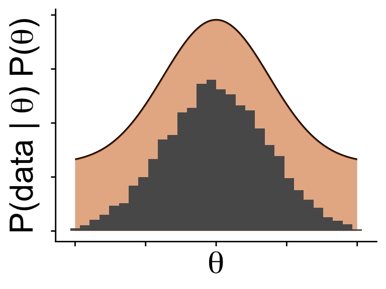
Use the shape of the posterior \(\mathbb{P}(\text{data} | \theta) \mathbb{P}(\theta)\) to draw a random sample consistent with the posterior
Monte Carlo (MC) can do this without a proper \(\mathbb{P}(\theta \mid \text{data})\)
by sampling values of \(\theta\) in proportion to height the of \(\mathbb{P}(\text{data} | \theta) \mathbb{P}(\theta)\)
So how do we get the posterior?
Use the shape of the posterior \(\mathbb{P}(\text{data} | \theta) \mathbb{P}(\theta)\) to draw a random sample consistent with the posterior
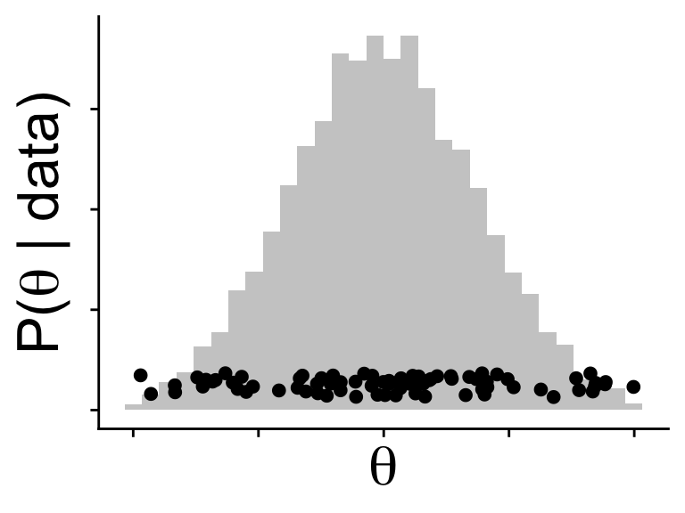
Sampling proportionately to \(\mathbb{P}(\text{data} | \theta) \mathbb{P}(\theta)\)
Yields a sample of \(\theta\)
That looks like it came from \(\mathbb{P}(\theta \mid \text{data})\)
Markov Chain Monte Carlo (MCMC)
MCMC is the method of choice for this task
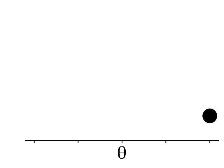
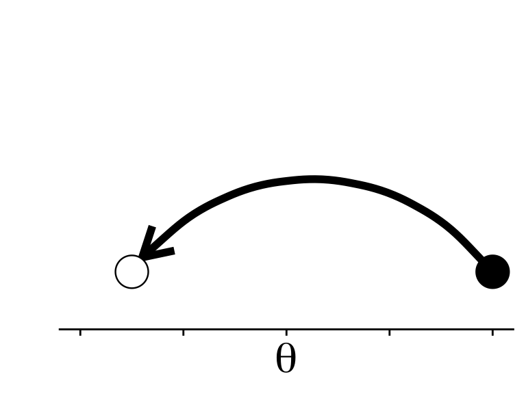
Start with an initial value for \(\theta\)
Somehow propose a new value using \(\mathbb{P}(\text{data} \mid \theta) \mathbb{P}(\theta)\)
Markov Chain Monte Carlo (MCMC)
MCMC is the method of choice for this task
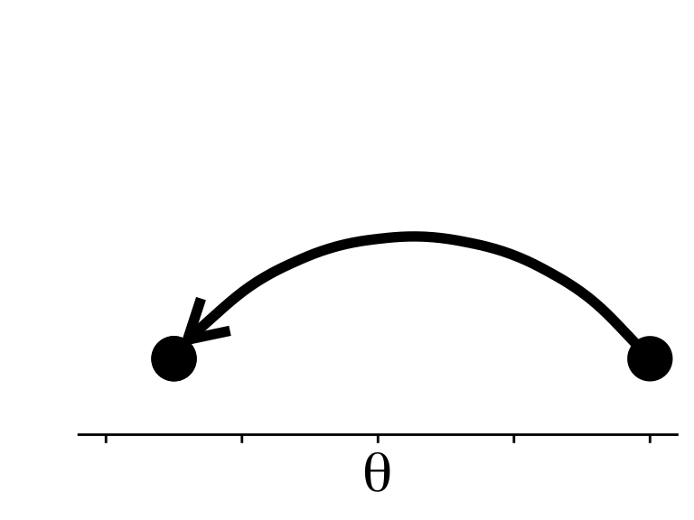
Repeat! with new value of \(\theta\) as starting point
Somehow propose a new value using \(\mathbb{P}(\text{data} \mid \theta) \mathbb{P}(\theta)\)
Do that enough and we get a sample from the posterior without ever knowing the equation for \(\mathbb{P}(\theta \mid \text{data})\)
Markov Chain Monte Carlo (MCMC)
MCMC is the method of choice for this task
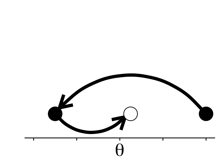
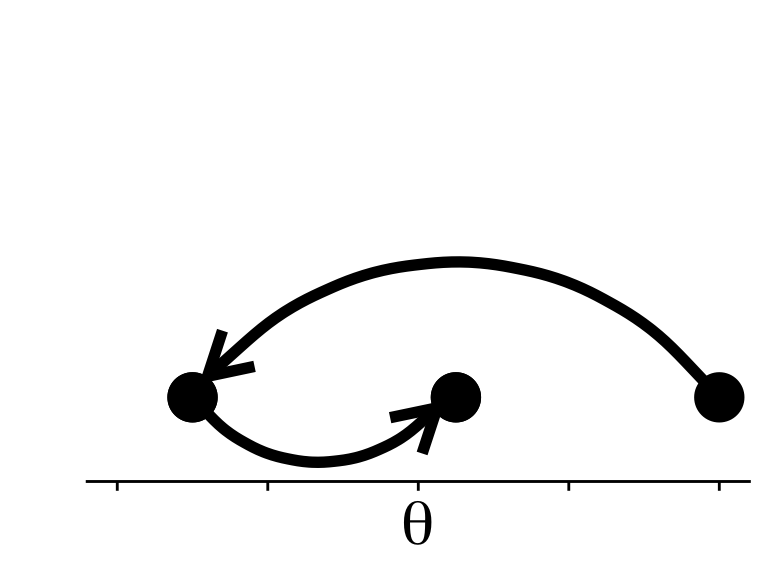
Repeat! with new value of \(\theta\) as starting point
Do that enough and we get a sample from the posterior…
…without ever knowing the equation for \(\mathbb{P}(\theta \mid \text{data})\)
Markov Chain Monte Carlo (MCMC)
Common MCMC algorithms include
Gibbs sampler
Metropolis-Hastings
random walk Metropolis
Hessian Monte Carlo
No-U-Turns (NUTS)
NUTS is what the software Stan uses, which is under the hood of the R code we’ll use
No-U-Turns algorithm
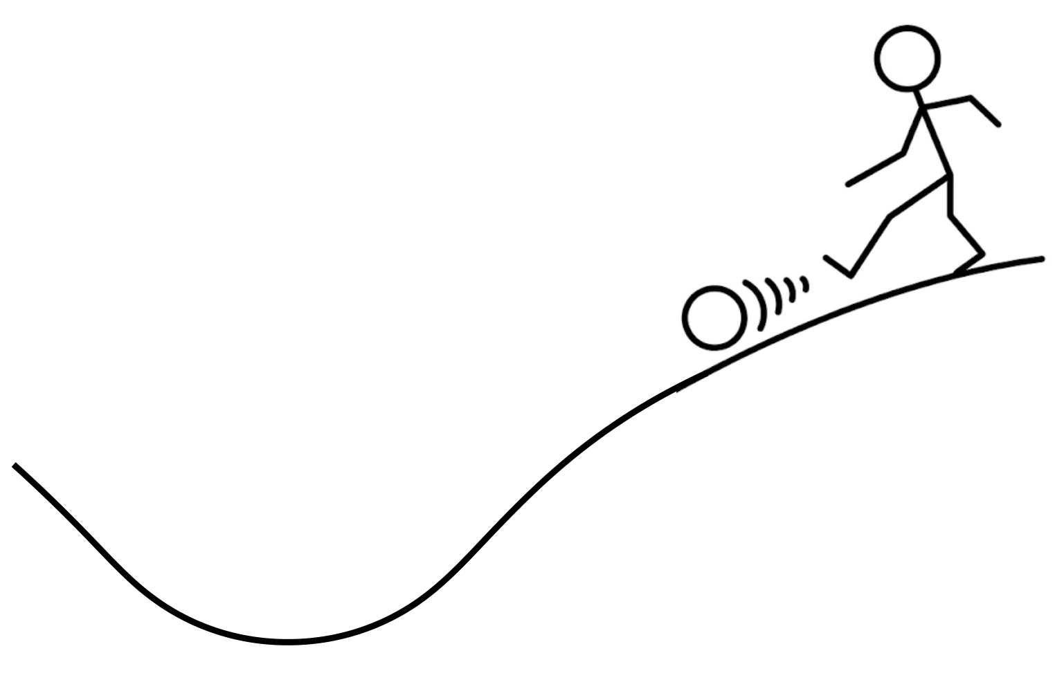
Imagine a kid kicking a ball in a hilly landscape
most of the time, the ball ends up at the bottom of a hill
No-U-Turns algorithm
A ball moving around the \(-\log(\mathbb{P}(\text{data} \mid \theta) \mathbb{P}(\theta))\) landscape according to the laws of physics is basically Hamiltonian MC
No-U-Turns just makes HMC more computationally efficient
No-U-Turns algorithm
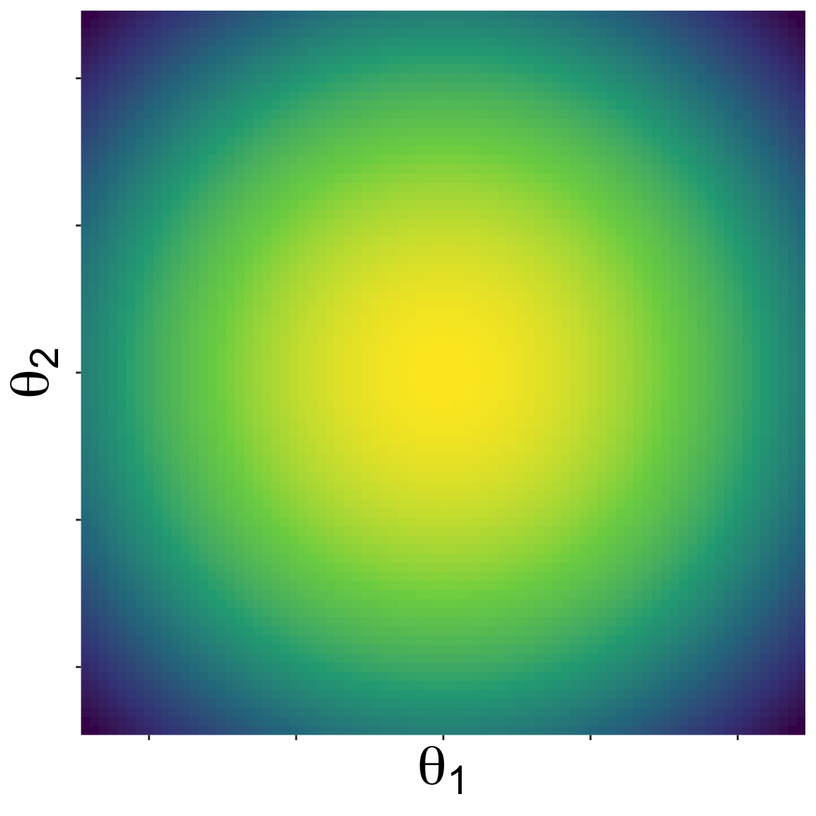
Here is a landscape with two parameters
No-U-Turns algorithm
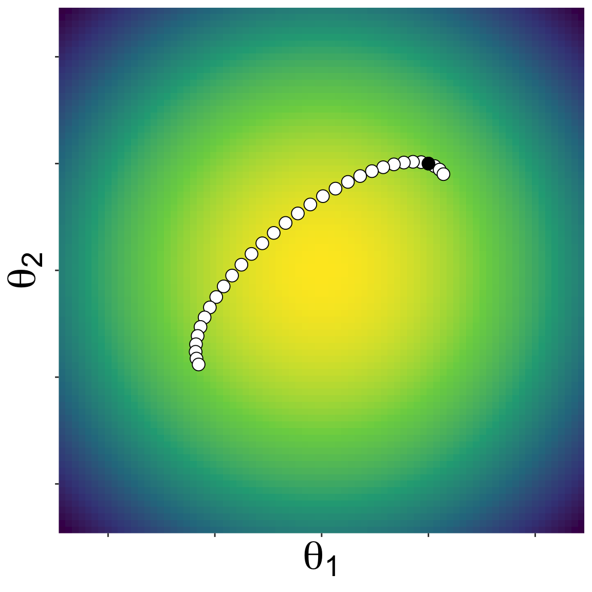
Starting from some initial location, NUTS proposes new parameter values by kicking a ball and seeing where it rolls on the landscape
No-U-Turns algorithm
A new set of parameter values along the path of the ball is randomly choosen, and the algorithm repeated
No-U-Turns algorithm
Eventually a sample of the posterior emerges
Package brms makes it easy for us
Despite the complexities of how this works under the hood, brms will make it feel familiar
library(brms)x <-runif(100, 0, 1)mu <-exp(-2+4* x)y <-rpois(length(x), mu)dat <-data.frame(x, y)m <-brm(y ~ x, data = dat, family =poisson(), prior =c(prior(normal(0, 1000), class = Intercept),prior(normal(0, 1000), class = b)))
Package brms makes it easy for us
Despite the complexities of how this works under the hood, brms will make it feel familiar