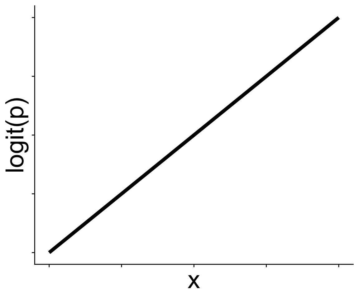
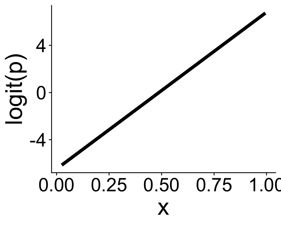
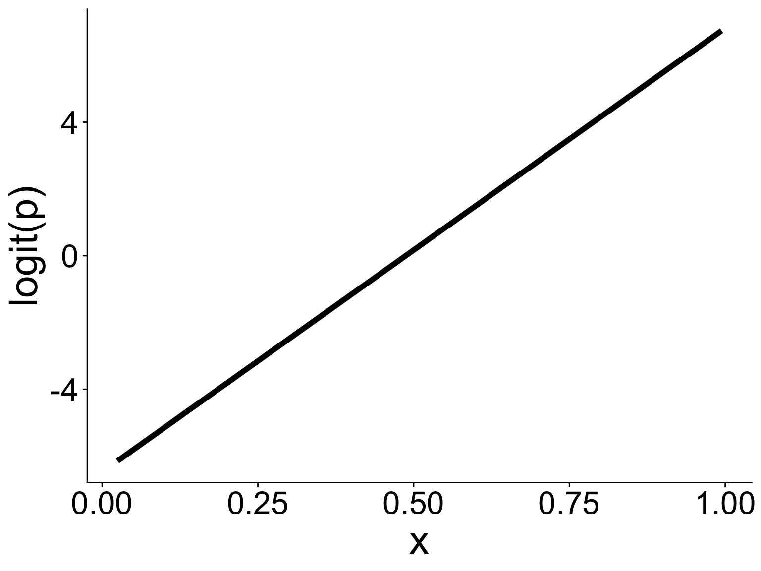
# get link function intercept and slopebb <-coefficients(mod)bb# write a function for the equationmy_probit <-function(x, intercept, slope) { intercept + slope * x}# use `geom_function`ggplot(data.frame(x =0:1, y =0:1), aes(x, y)) +geom_function(fun = my_probit, args =list(intercept = bb[1], slope = bb[2])) +ylab("logit(p)")
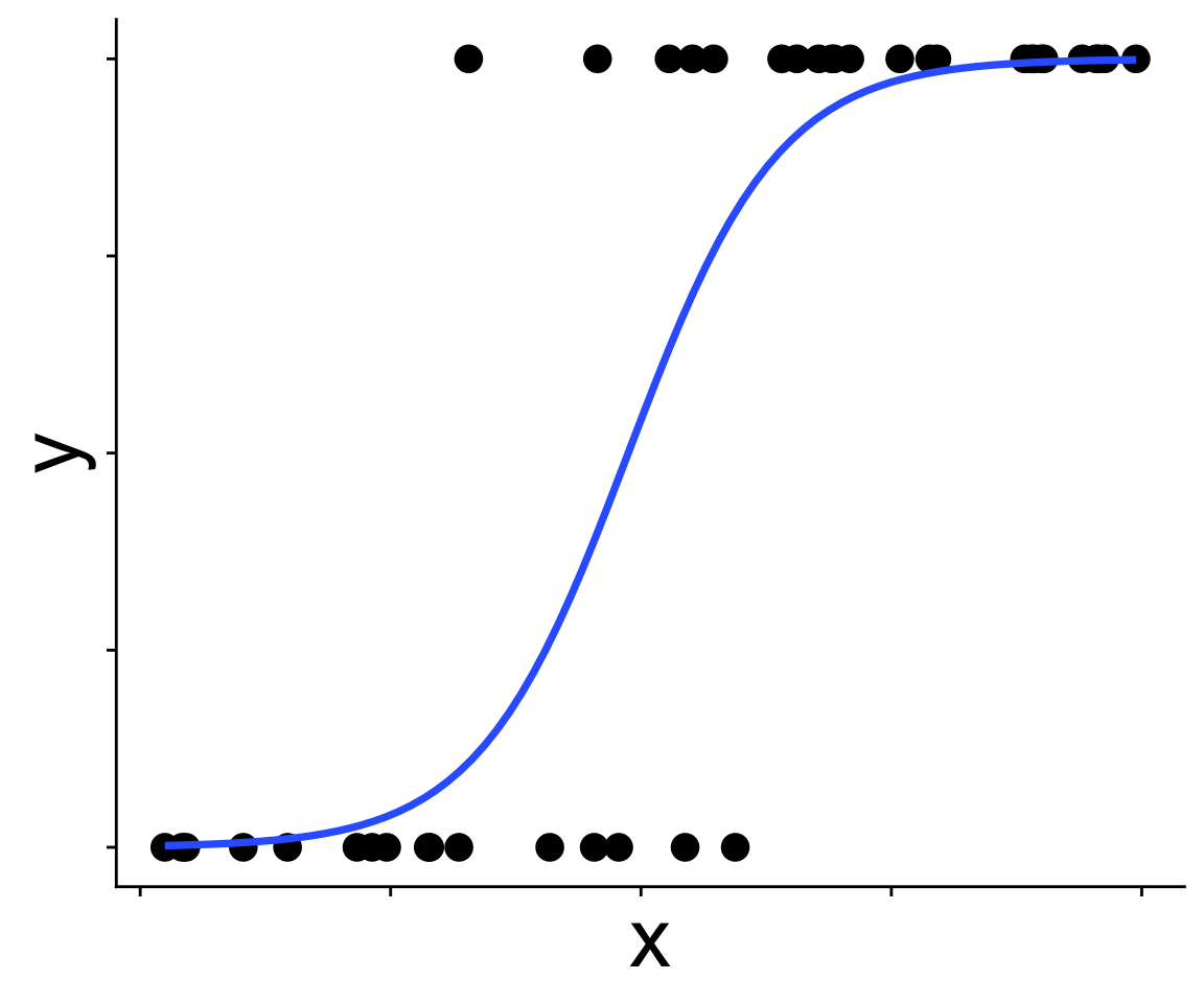
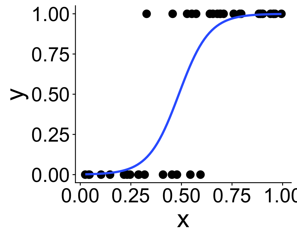
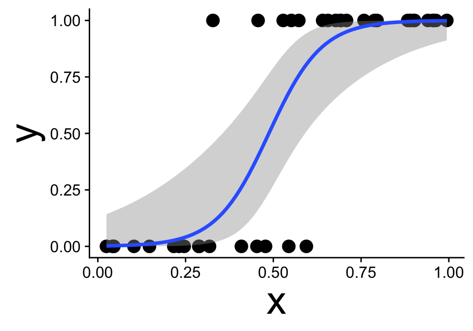
Visualizing the model and data
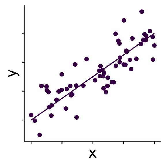
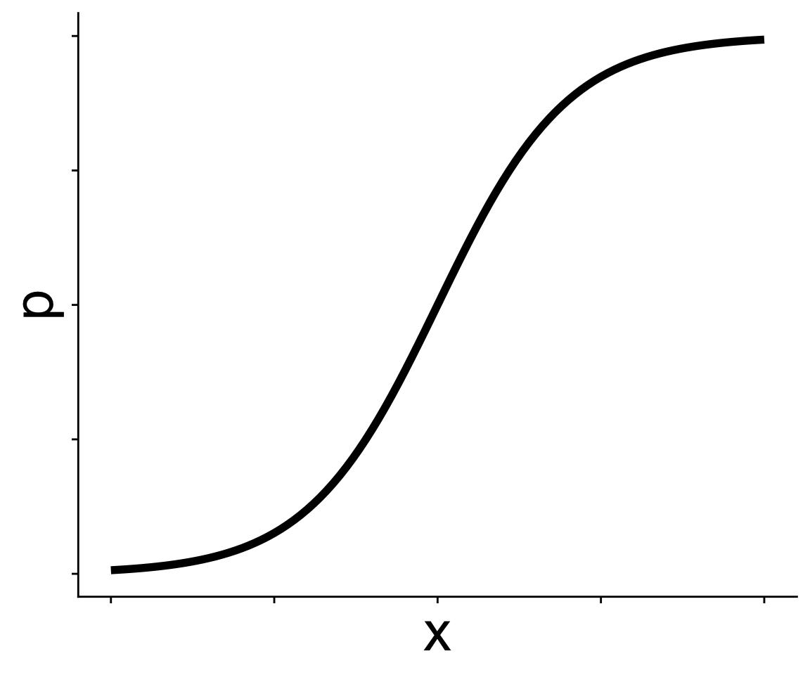
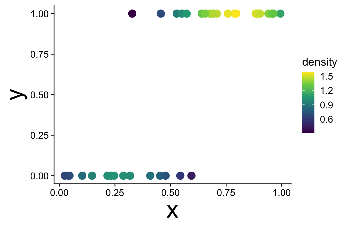
Let’s look at the link function in two ways
With the predicted values for logit(p)
# function `predict` gives us model predictions# `type = link` says, give us predictions on link function scalelogitp_hat <-predict(mod, type ="link")head(logitp_hat)# add a column for logit(p) and you're ready to plot!ggplot(mutate(dat, logitp = logitp_hat), aes(x, logitp)) +geom_line(linewidth =2) +ylab("logit(p)")
Visualizing the model and data
Either way gives you this graph
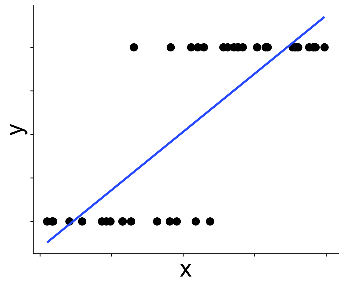
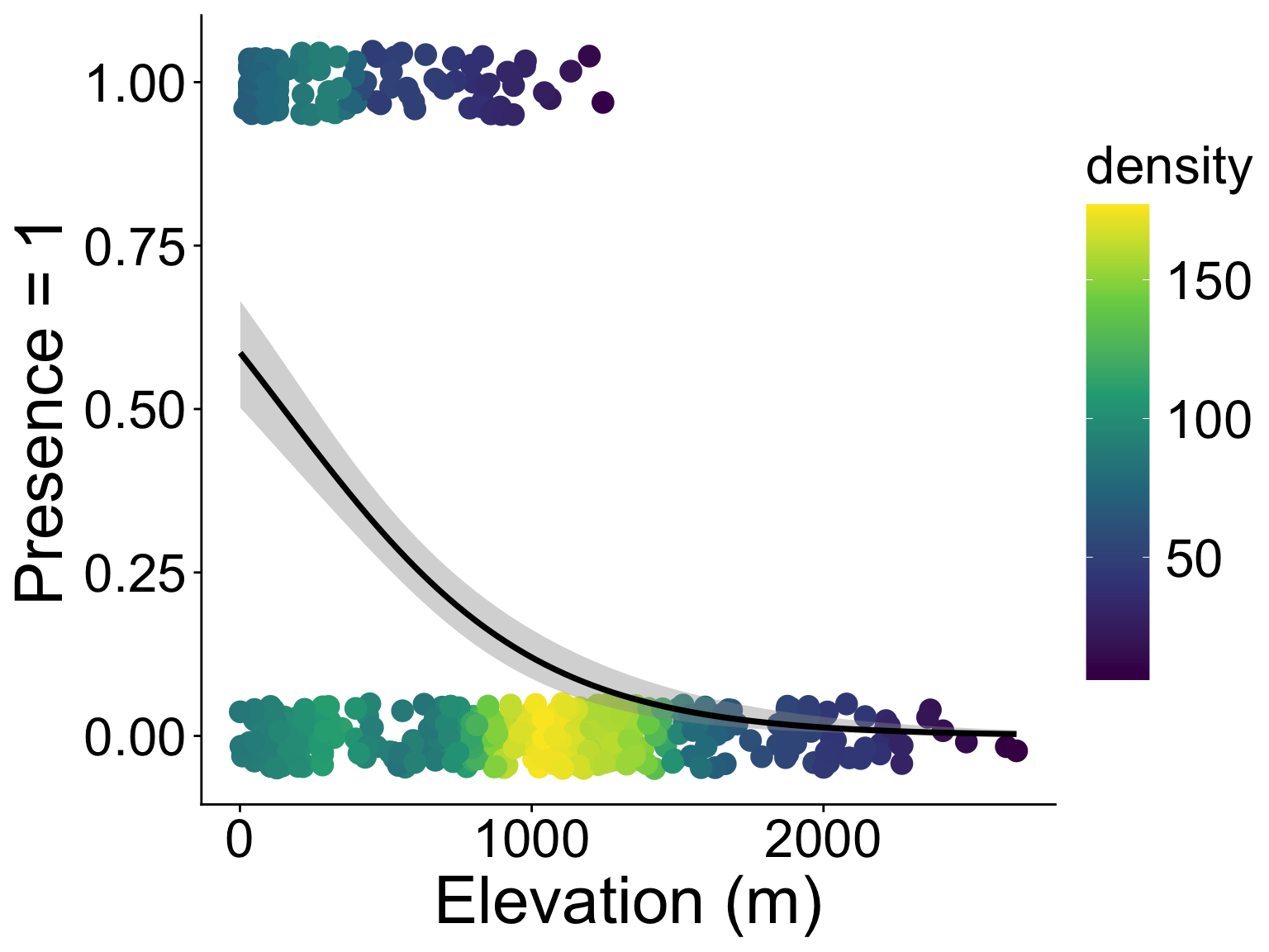
Binomial GLM: Use cases
presence/absence, e.g., where is the strawberry guava?
# i did some data prep alreadyhead(stra_gua) |>kable()
PlotID
elev_m
any_gua
num_gua
num_tre
1
395.1798
1
6
75
2
129.6578
1
6
80
3
129.6578
0
0
37
4
129.6578
1
50
100
5
129.6578
1
49
99
6
129.6578
1
1
64
glm(any_gua ~ elev_m,
    data = stra_gua,
    family = binomial)
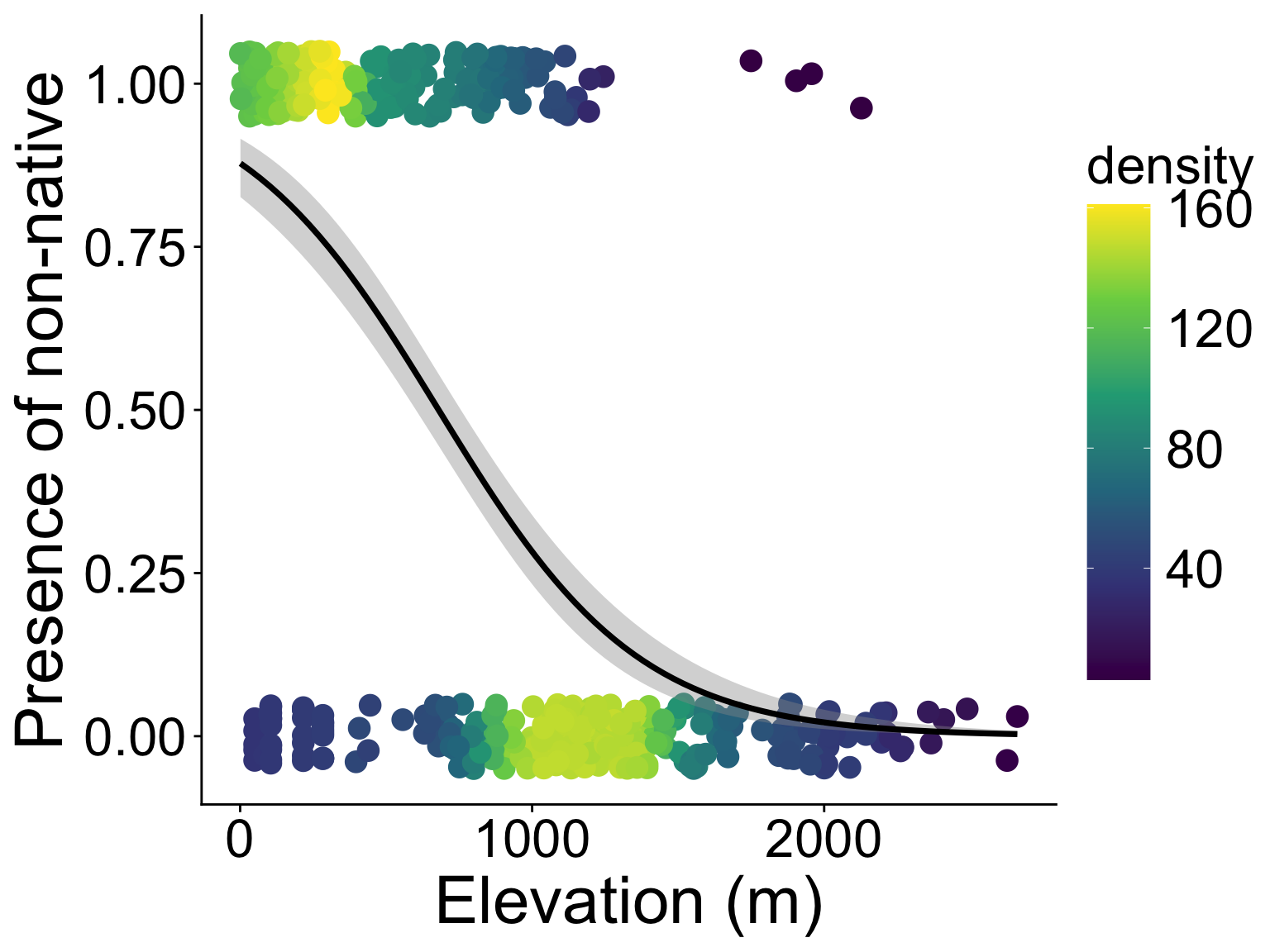
Binomial GLM: Use cases
binary property, e.g., non-native or native?
# i did some data prep alreadyhead(tree_plot) |>kable()
PlotID
elev_m
any_non
num_non
num_tre
1
395.1798
1
9
75
2
129.6578
1
7
80
3
129.6578
1
1
37
4
129.6578
1
56
100
5
129.6578
1
49
99
6
129.6578
1
23
64
glm(any_non ~ elev_m, data = tree_plot, family = binomial)coefficients(mn)
Binomial GLM: Use cases
binary property, wait, aren’t we wasting tree-level data?
# i did some data prep alreadyhead(tree_stem) |>kable()
PlotID
elev_m
non_nat
2
129.6578
0
2
129.6578
0
2
129.6578
0
2
129.6578
0
2
129.6578
0
2
129.6578
0
glm(non_nat ~ elev_m,
    data = tree_stem,
    family = binomial)
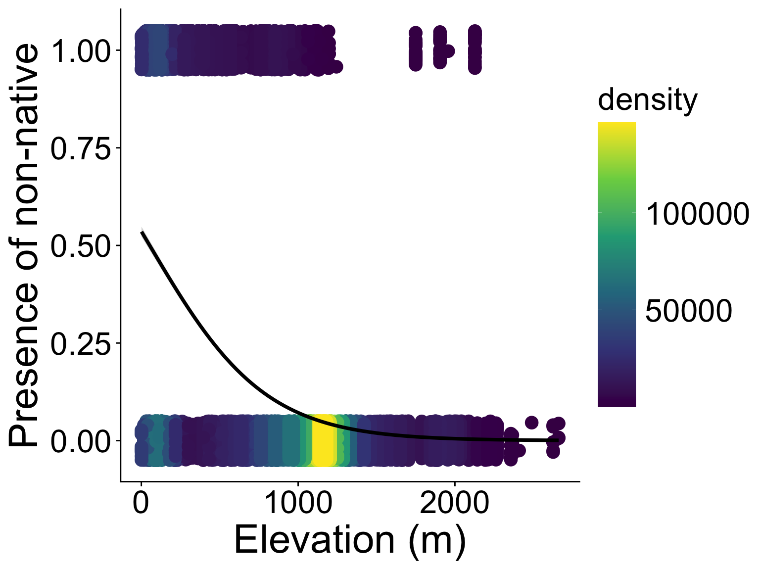
Binomial GLM: Use cases
binary property, e.g., non-native or native?
No that wasn’t a good idea—pseudo replication in plots
But before you go thinking of random effects
Remember, within each plot is like a binomial sample:
“successes”: number of non-native trees
total size: number of all trees
Binomial GLM: Use cases
number of successes vs. failures, back to plot-level data
head(tree_plot) |>kable()# hint: scroll right
PlotID
elev_m
any_non
num_non
num_tre
1
395.1798
1
9
75
2
129.6578
1
7
80
3
129.6578
1
1
37
4
129.6578
1
56
100
5
129.6578
1
49
99
6
129.6578
1
23
64
# wants a matrix (from cbind) of num success and num failureglm(cbind(num_non, num_tre - num_non) ~ elev_m, data = tree_plot, family = binomial)
Plotting is more convoluted so let’s go into it more
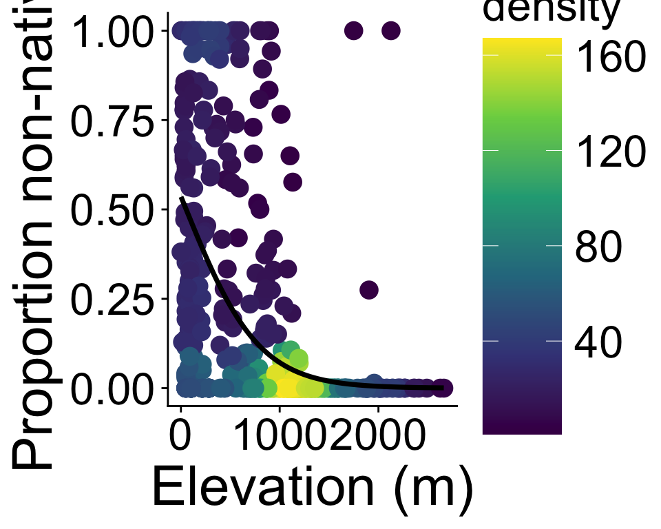
Binomial GLM: Use cases
number of successes vs. failures, back to plot-level data
ggplot(tree_plot, aes(elev_m, num_non / num_tre, # include `success` and `failure`# for use in `geom_smooth`success = num_non, failure = num_tre - num_non)) +geom_pointdensity() +scale_color_viridis_c() +geom_smooth(method ="glm", color ="black",# need to add a specific formulaformula =cbind(success, failure) ~ x,method.args =list(family = binomial))
Binomial GLM: Use cases
number of successes vs. failures, back to plot-level data