Likelihood Ratio Tests and Confidence Intervals

Is overdispersion supported by my data?

We saw that the Poisson GLM assumes variance = mean = \(\lambda\)

A negative binomial GLM relaxes that: variance \(= \lambda + \lambda^2 / k\), where \(k\) is an extra dispersion parameter

mod_pois <- glm(nspp ~ log(Plot_Area),
                data = dat_plt, family = poisson)

mod_nb <- glm.nb(nspp ~ log(Plot_Area),
                 data = dat_plt)

Both models fit. But is the negative binomial actually better?

Is overdispersion supported by my data?

We can compare log likelihoods

logLik(mod_pois)

'log Lik.' -1185.718 (df=2)

logLik(mod_nb)

'log Lik.' -1162.635 (df=3)

The negative binomial has a higher log likelihood, but is that difference significant?

What to consider for significance

Quantify the difference between models
Compare that quantity to what we would expect if there were no real difference, i.e. the null

What is the null?

If the two models were truly equivalent (no overdispersion, \(k \rightarrow \infty\)), what would the difference in log likelihoods look like?

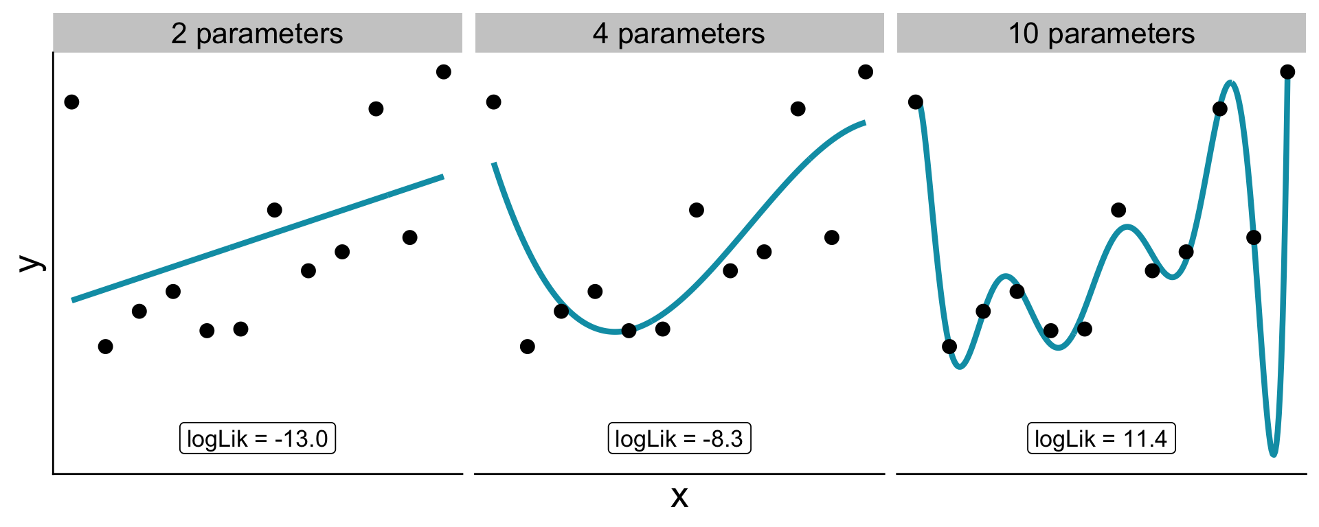
Adding a parameter always increases log likelihood a little, even when fitting noise
If the null is true, the gain is just random luck

We need a null distribution for accidental log likelihood gains

What is the null?

Need to consider: more parameters let the model bend to match idiosyncrasies of the data, even pure noise (the case here)

What is the null?

How do more parameters increase likelihood?

Access to higher parameter dimensions.

Log likelihoods are approximately quadratic

Thus vertical distances are squared

What is the null?

If vertical distances are squared

\(2(\log\mathscr{L}(\text{data} \mid b_0,~b_1) - \log\mathscr{L}(\text{data} \mid b_0)) \sim \chi^2\)

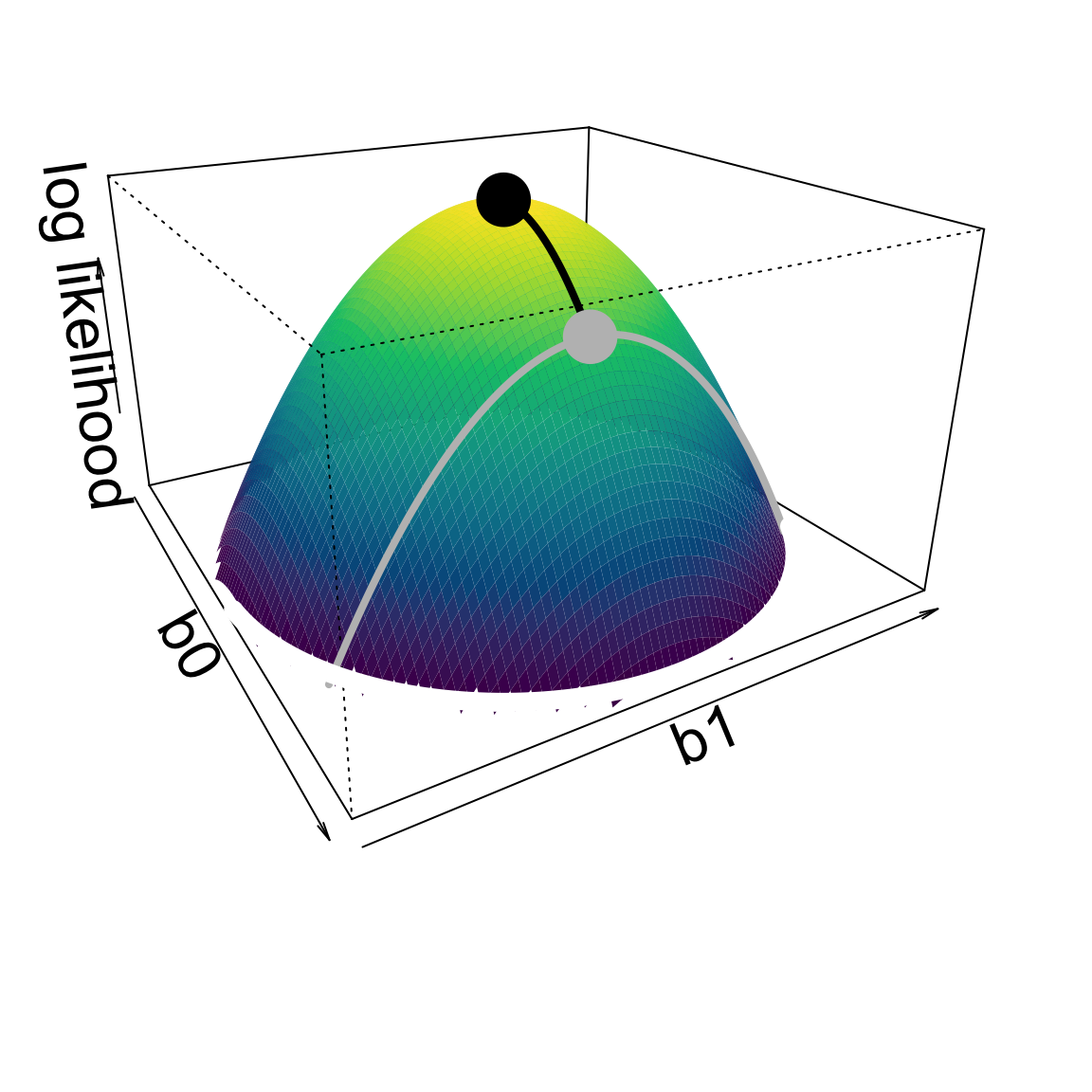
differences in log likelihoods between models (times 2) will be \(\chi^2\)-distributed

the times 2 is a scaling factor from deep in the math

The likelihood ratio test

This \(\chi^2\) distribution provides our null, and gives us a significance test!

\[ \Lambda = 2\!\left(\log\mathscr{L}_\text{full} - \log\mathscr{L}_\text{null}\right) \;\sim\; \chi^2_{df} \]

\(df\) = difference in number of parameters between models
If the added parameters are truly meaningful, \(\Lambda\) should be large and we should reject the null

LRT applied to overdispersion

ll_pois <- logLik(mod_pois)
ll_nb <- logLik(mod_nb)

Lambda <- 2 * (ll_nb - ll_pois)
Lambda

'log Lik.' 46.16588 (df=3)

# negative binomial has one extra parameter (k)
pchisq(Lambda, df = 1, lower.tail = FALSE)

'log Lik.' 1.086526e-11 (df=3)

LRT applied to overdispersion

We can also use the built-in anova function:

anova(mod_pois, mod_nb, test = "Chisq")

Analysis of Deviance Table

Model 1: nspp ~ log(Plot_Area)
Model 2: nspp ~ log(Plot_Area)
  Resid. Df Resid. Dev Df Deviance Pr(>Chi)
1       526     751.31                     
2       526     515.85  0   235.46

LRT: key assumption

Nested models

The LRT requires the null model to be a special case of the full model

Poisson is nested in negative binomial (\(k \to \infty\) recovers Poisson)
glm(y ~ x) is nested in glm(y ~ x + z)
Not nested: Poisson vs. normal; two models with non-overlapping predictors

LRT for a predictor: does human impact matter?

After accounting for area, does human impact (hii) improve the fit?

mod_nb_area <- glm.nb(nspp ~ log(Plot_Area), data = dat_plt)
mod_nb_area_hii <- glm.nb(nspp ~ log(Plot_Area) + hii, data = dat_plt)

logLik(mod_nb_area)

'log Lik.' -1162.635 (df=3)

logLik(mod_nb_area_hii)

'log Lik.' -1153.187 (df=4)

LRT for a predictor: does human impact matter?

anova(mod_nb_area, mod_nb_area_hii, test = "Chisq")

Likelihood ratio tests of Negative Binomial Models

Response: nspp
                 Model     theta Resid. df    2 x log-lik.   Test    df
1       log(Plot_Area)  9.014755       526       -2325.269             
2 log(Plot_Area) + hii 10.079784       525       -2306.374 1 vs 2     1
  LR stat.      Pr(Chi)
1                      
2 18.89501 1.381132e-05

anova with test = "Chisq" does the LRT for us when comparing nested glm objects

One extra parameter (hii), so \(df = 1\)

LRT for a predictor: interpreting the result

coefficients(mod_nb_area_hii)

   (Intercept) log(Plot_Area)            hii 
   -2.17062071     0.50678811     0.01335919

Despite the slope for hii being small (and positive), \(P\)-value is less than 0.05

Confidence intervals as another way to evaluate significance

A coefficient is judged significant if its confidence interval does not include zero

Two ways to build CIs from likelihood:

Likelihood ratio interval — invert the LRT
Wald interval — use the CLT approximation directly

LRT confidence interval

Find all values of \(\theta\) such that the LRT would not reject the null \(H_0: \theta = \theta_0\)

\[ 2\!\left(\log\mathscr{L}(\hat\theta) - \log\mathscr{L}(\theta_0)\right) \leq 3.84 \]

Rearranging:

\[ \log\mathscr{L}(\theta_0) \geq \log\mathscr{L}(\hat\theta) - 1.92 \]

LRT confidence interval

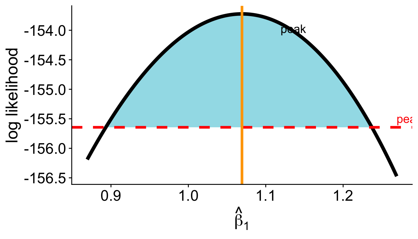
LRT confidence interval

In R, confint on a glm uses this profile likelihood approach by default:

confint(mod_nb_area_hii)

                      2.5 %      97.5 %
(Intercept)    -2.856145450 -1.50666094
log(Plot_Area)  0.409973650  0.60677711
hii             0.007402642  0.01929201

Wald confidence intervals

Another approach: use the CLT approximation directly

According to CLT \(\hat\theta\) is approximately normally distributed:

\[ \hat\theta \pm z_{0.975} \cdot \widehat{\text{SE}}(\hat\theta) \]

confint.default(mod_nb_area_hii)

                      2.5 %      97.5 %
(Intercept)    -2.846644217 -1.49459721
log(Plot_Area)  0.408126031  0.60545018
hii             0.007530585  0.01918779

confint.default uses the Wald approach — fast but less accurate

LRT vs. Wald intervals

LRT (profile likelihood)

more accurate, especially for small \(n\)
CI can be asymmetric — follows the actual shape of the likelihood surface

Wald

fast and simple
symmetric by construction
less accurate when log likelihood surface is asymmetric

Summary

The LRT compares nested models: \(\Lambda = 2(\log\mathscr{L}_\text{full} - \log\mathscr{L}_\text{null}) \sim \chi^2_{df}\)
The \(\chi^2\) null distribution arises from the CLT applied to MLE — the log likelihood surface is approximately quadratic
Nested models are required: null must be a special case of full
anova(mod1, mod2, test = "Chisq") does the work in R

Summary

LRT confidence intervals invert the LRT: all \(\theta\) within 1.92 log likelihood units of the peak form the 95% CI
Wald intervals use the normal approximation directly