The Poisson Generalized Linear Model

Consider the Poisson distribution…

\[ y \sim \text{Pois}(\lambda) \]

Often used to model counts of things (number of trees, number of species, etc.)

\(\lambda\) is both the mean and the variance of the distribution

Consider the Poisson distribution…

\(\lambda\) is both the mean and the variance of the distribution.
What must be true about \(\mathbf{\lambda}\)?

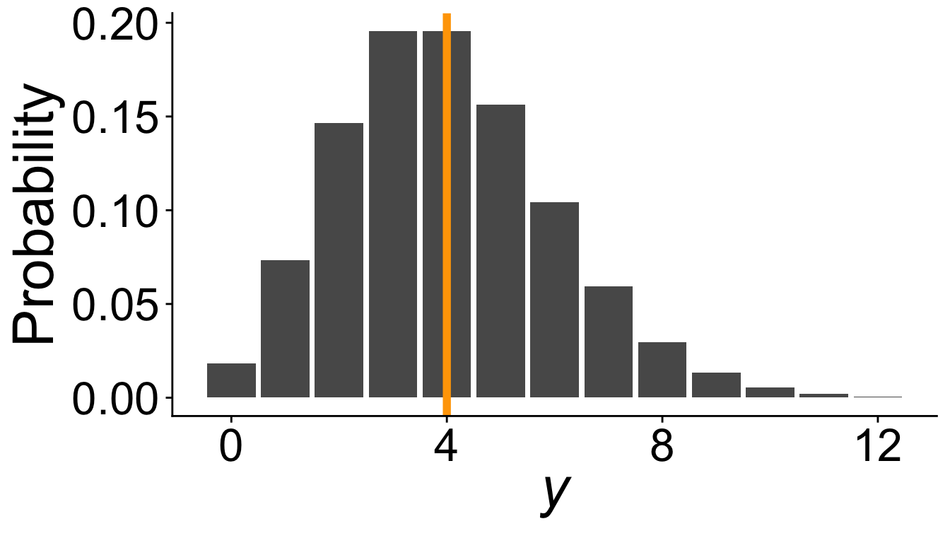
must be true: \(\lambda \geq 0\)

Consider the Poisson GLM…

If we wanted to use a Poisson distribution in a GLM, we have to make sure \(\lambda \geq 0\)

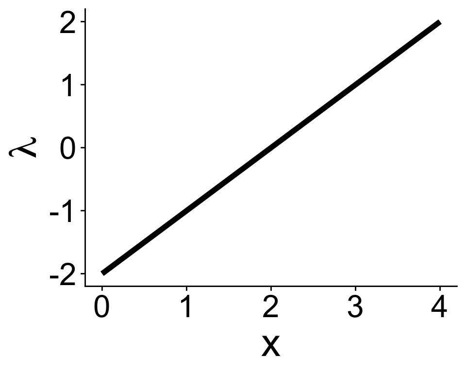
Can’t have this

\[ \lambda = b_0 + b_1 x \]

Need some kind of link function

Consider the Poisson GLM…

If we wanted to use a Poisson distribution in a GLM, we have to make sure \(\lambda \geq 0\)

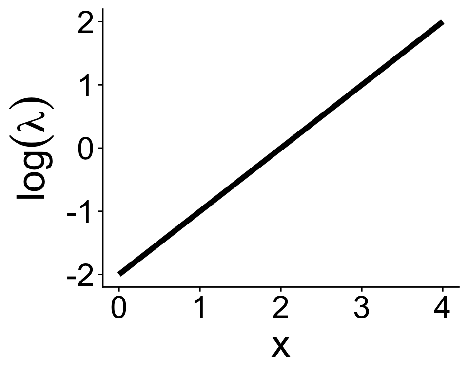
\(e^\text{anything} \geq 0\), always

\[ \lambda = e^{b_0 + b_1 x} \]

And the inverse gives us back the straight line

\[ \log(\lambda) = b_0 + b_1 x \]

So with Poisson GLM, a log link function is the default

Poisson GLM with glm function in R

Back to species area

\[ \begin{aligned} S &= cA^z \\ \log(S) &= \log(c) + z\log(A) \end{aligned} \]

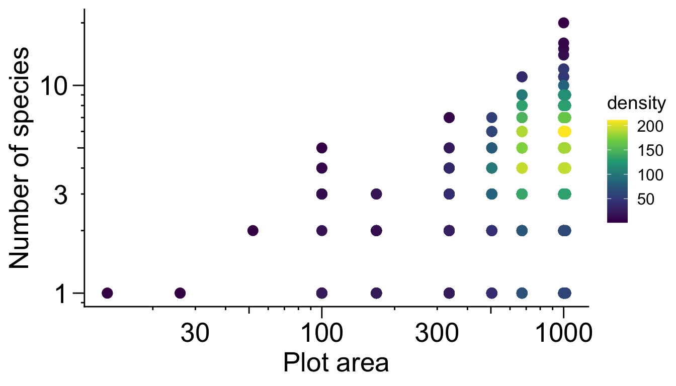
(note: 2 super large plots excluded)

lends itself to a log link function

\[ \begin{aligned} \bar{S} &= \lambda \\ \log(A) &= x \\ \Rightarrow \log(\bar{S}) &= b_0 + b_1 \log(A) \end{aligned} \]

Poisson GLM with glm function in R

with data like these

Plot_Area	nspp
1000.00	9
1017.88	9
1017.88	2
1017.88	9
1017.88	4
1017.88	9

can fit a Poisson model like this

sar <- glm(nspp ~ log(Plot_Area), 
           data = dat_plt, 
           family = poisson)

recall: the link function already takes care of logging the mean species richness, no need to log again

coefficients(sar)

   (Intercept) log(Plot_Area) 
    -1.8086075      0.4893528 

What besides area?

• We are probably interested in more than area
• Area might even be a “nuisance variable”
  • one that we have to account for
  • but we’re more interested in other variables
• How about hii (human impact) and avg_temp_annual_c (temperature)?
• Can!

Adding more explanatory variables

mod <- glm(nspp ~ log(Plot_Area) + hii + avg_temp_annual_c, 
           data = dat_plt, 
           family = poisson)

coefficients(mod)

      (Intercept)    log(Plot_Area)               hii avg_temp_annual_c 
     -2.320992411       0.516567381       0.011011301       0.007295895 

After accounting for area, species richness increases (weakly) with both human impact and temperature

Perhaps non-native plants augment species richness (Sax & Gaines 2003)

Or perhaps lowland (i.e. hot) forests were incredibly diverse (Rock 1913) and are now lost to heavy human modification

Adding more explanatory variables

Beyond biological interpretation, adding more variables requires care

This is the likelihood surface for our model, visualizing just the coefficients for human impact and temperature

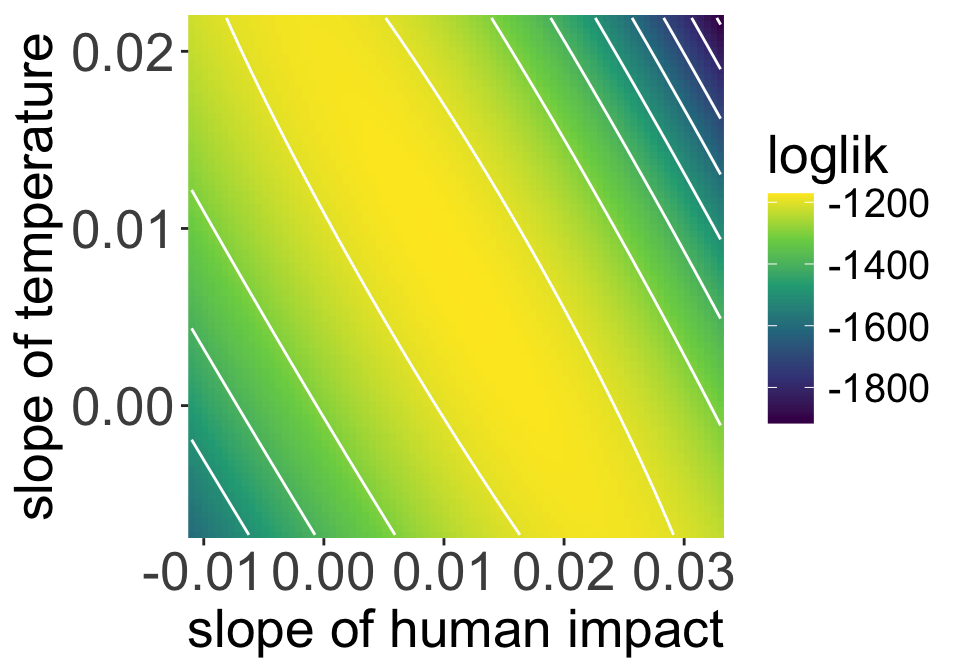
There is a long, flat ridge across the likelihood surface

That’s a problem because it is difficult and unreliable to figure out the optimal parameter combination

why?

Adding more explanatory variables

Collinearity creates these kinds of ridges

Human impact and temperature are correlated

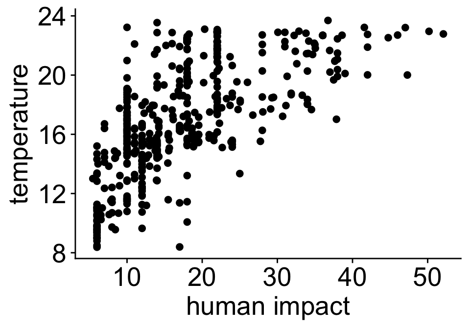
Check for collinearity, a common cut off is \(-0.6 < r < 0.6\)

References

Rock JF. 1913. The indigenous trees of the hawaiian islands. Patronage, Honoulu: Hawaii.

Sax DF, Gaines SD. 2003. Species diversity: From global decreases to local increases. Trends in Ecology & Evolution 18:561–566. Elsevier.