Introducing probability

Probability in ecology and evolution

pick a random grid cell with equal probability
replace with either:
- dispersal from metacommunity with probability \(m\), …or…
- local birth with probability \(1 - m\)
choose replacement individual with equal probability
replacement undergoes speciation with probability \(\nu\)

Probability in ecology and evolution

This “game” is a simplified version of Hubbell’s (2001) Unified Neutral Theory of Biodiversity (UNTB)
Even the full theory is a simplification of the real world, but can still predict, with surprising accuracy, properties of biodiversity like the species abundance distribution
UNTB and other models shows us the importance of probability and randomness

Probability in ecology and evolution

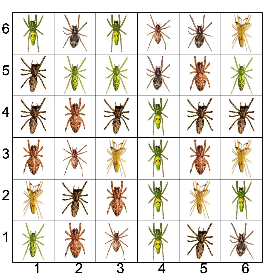
How could we play this “game” using just two 6-sided dice?

Let:

\(m = \frac{1}{3}\)
\(\nu = \frac{1}{36}\)

Rules of probability

We learned some in the game

Probabilities sum to 1 (something has to happen)
Probabilities add (prob. this or that = \(\mathbb{P}(this) + \mathbb{P}(that)\))
Probabilities multiply (prob. this and that = \(\mathbb{P}(this) \mathbb{P}(that)\))
But not always…

…Consider this: probability of speciation \(\nu = 1/12\)

Rules of probability

Consider this: probability of speciation \(\nu = 1/12\)

Can achieve this with sum of two dice = 4

1 + 3 = 4 (prob = 1/36)

2 + 2 = 4 (prob = 1/36)

3 + 1 = 4 (prob = 1/36)

Total prob = 3/23 = 1/12

Rules of probability

Consider this: probability of speciation \(\nu = 1/12\)

A probability tree can help

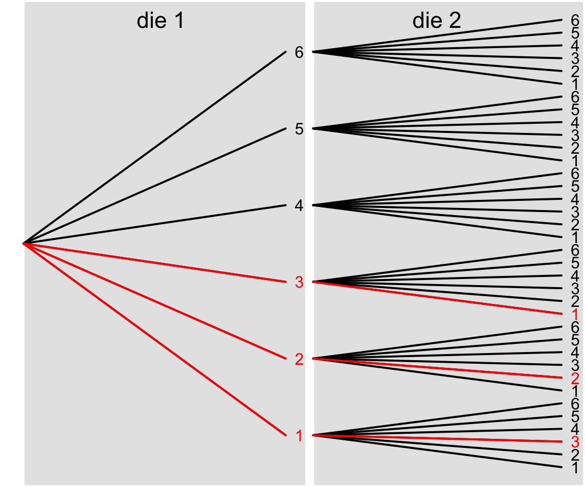
Count up the ways to get sum of two dice = 4, divide by total number of combinations

Rules of probability

Consider this: probability of speciation \(\nu = 1/12\)

Imagine: speciation occurred! What is the probability the first dice was 2 or less?

Can no longer simply add \(\mathbb{P}(1) + \mathbb{P}(2) = 2/6 = 1/3\)
Use the probability tree

This is conditional probability: probability of first die \(\leq2\) given sum of two dice is 4

\[ \mathbb{P}(die_1 \leq 2 \mid sum = 4) \]

Rules of probability

Consider this: probability of speciation \(\nu = 1/12\)

Imagine: speciation occurred! What is the probability the first dice was 2 or less?

\[ \mathbb{P}(die_1 \leq 2 \mid sum = 4) = \frac{2}{3} \]

Counting still works, but the condition changes the space over which we count

Rules of probability

Consider this: probability of speciation \(\nu = 1/12\)

We can also use math to help us “count” given a condition

\[ \begin{align} &\mathbb{P}(die_1 \leq 2 \mid sum = 4) \\ &= \frac{\mathbb{P}(die_1 \leq 2~\&~sum = 4)}{\mathbb{P}(sum = 4)} \\ &= \frac{2/36}{3/36} \\ &= \frac{2}{3} \end{align} \]

Rules of probability

Probabilities sum to 1 (something has to happen)
For independent events:
- Probabilities add
  (prob. this or that = \(\mathbb{P}(this) + \mathbb{P}(that)\))
- Probabilities multiply
  (prob. this and that = \(\mathbb{P}(this) \mathbb{P}(that)\))
For non-independent events conditional probabilities apply
- \(\mathbb{P}(A \mid B)\) means “prob. of A given B”
- \(\mathbb{P}(A \mid B) = \frac{\mathbb{P}(A \& B)}{\mathbb{P}(B)}\)

Rules of probability

Just a note:

Don’t confuse \(\mathbb{P}(A \mid B)\) notation (which means “A given B”) with code notation A|B (which means “A or B”)

Probability as couning and as frequency

We have already seen that probability can result from counting

Probability as couning and as frequency

Probability also can result from long term frequency:

If I ran our “game” 10,000 times and recorded 831 dispersal events, what would you guess would be \(\mathbb{P}(\text{dispersal}) = m\)?

Probability as couning and as frequency

Probability also can result from long term frequency:

If I ran our “game” 10,000 times and recorded 831 dispersal events, what would you guess would be \(\mathbb{P}(\text{dispersal}) = m\)?

831 / 10000

[1] 0.0831

So maybe I was playing with the rules \(m = 1/12\) (which is about 0.0833)

Random variables and probability distributions

The number of dispersal events is an example of a random variable
Its value from one game to the next is not fixed but random
You could imagine millions of random variables
- The number of species present in an area
- The abundance of an arbitrary species (these two r.v.’s are indeed predicted by UNTB)
- The diameter at breast height of an arbitrary tree

Random variables and probability distributions

Random variables can be described with probability distributions

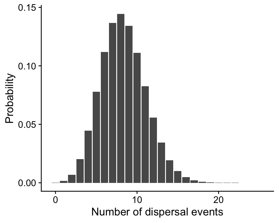
Here is an example for 100 iterations and \(m = \frac{1}{12}\)

Technically the \(r.v.\) could go all the way to 100 on the x-axis, but the probability of that many dispersal events is vanishingly small

Random variables and probability distributions

Here is an example for 100 iterations and \(m = 1/12\)

This is a probability mass function because the height of the bars really are probabilities

Random variables and probability distributions

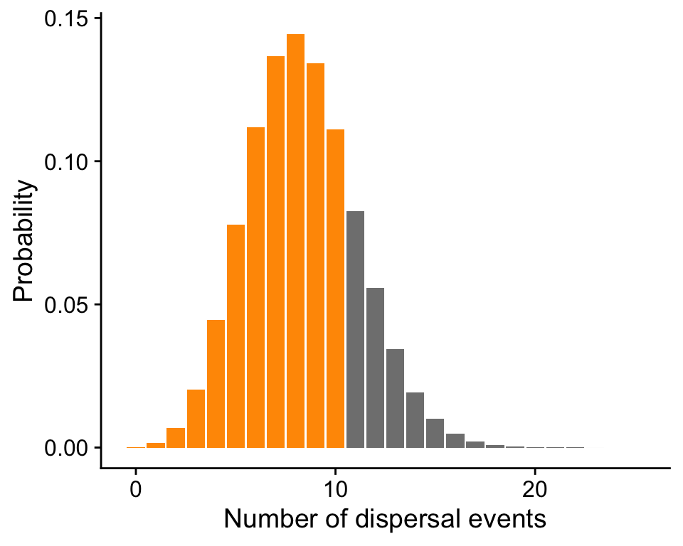
We can add heights of bars to calculate probabilities over ranges of values:

\[ \begin{align} \mathbb{P}(n \leq 10) &= \sum_{i = 0}^{10} \mathbb{P}(n = i) \\ &= 0.79 \end{align} \]

Random variables and probability distributions

We emphasized this is a probability mass function (PMF) because heights of bars are actual probabilities

This applies when the r.v. is discrete (e.g. an integer)

Random variables and probability distributions

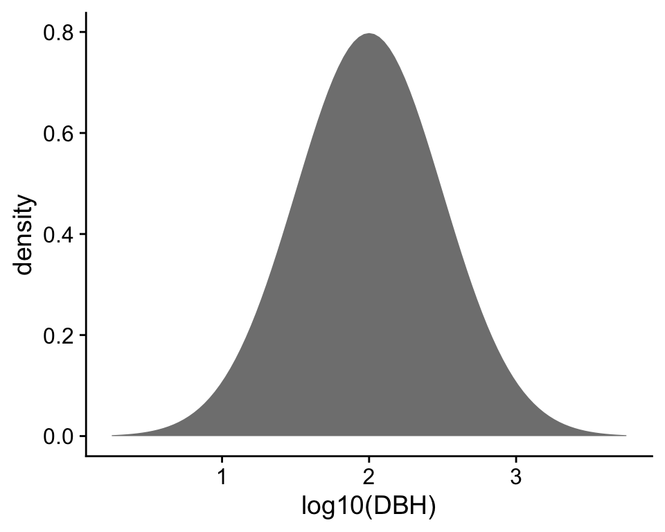
For a continuous r.v. like diameter at breast height, the y-axis is not equal to probability because \(\mathbb{P} \rightarrow 0\) for a continuous value with infinite precision

Instead we think of probability density and thus a probability density function (PDF)

Random variables and probability distributions

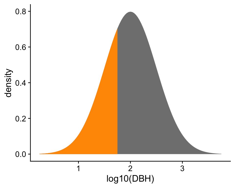
If we “add up” (technically integrate) the area under the PDF curve we again arrive at a real probability

e.g., according to this PDF \(\mathbb{P}(\log_{10}(DBH) \leq 1.75) = 0.309\)

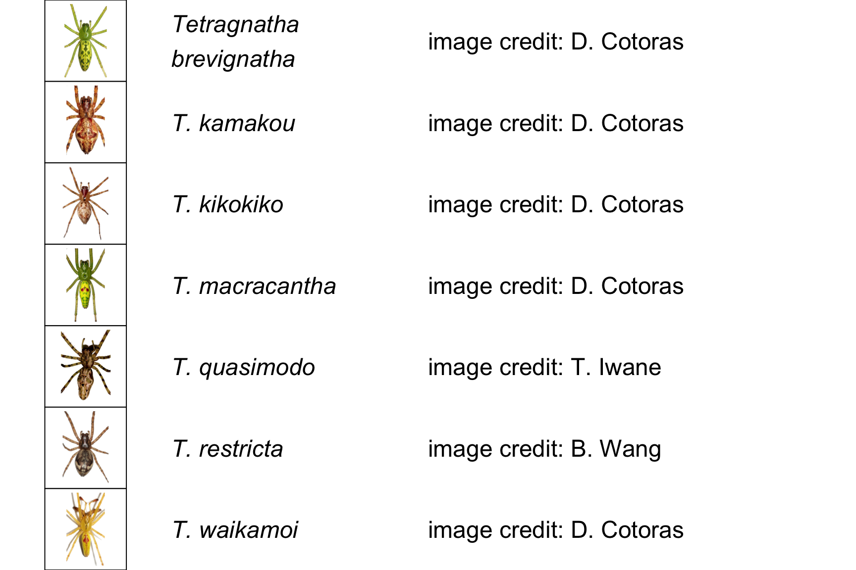
Spider image credits

References

Hubbell SP. 2001. The unified neutral theory of biodiversity and biogeography. Princeton University Press.