# uniformly distributed explanatory variable
x <- runif(100)

# calculate the mean of `y` as a function of `x`
# (don't worry about interpreting the right hand side right now)
lambda <- exp(1 + 2 * x)

# finally calculate `y`
y <- rpois(length(x), lambda)

# combine `x` and `y`
dat <- data.frame(x = x, y = y)1 Likelihood, AIC, and likelihood ratio tests
1.1 Let’s start with a model
Let’s start with a Poisson GLM and a made-up dataset to go along with it. Our data will just be y (the response variable) and x (the explanatory variable). We will assume y is the count of something (e.g. species abundance) and x is some kind of continuous numerical variable like temperature or rainfall, etc.
Let’s simulate some data
Here’s the first few rows of our simulated data
| x | y |
|---|---|
| 0.2875775 | 5 |
| 0.7883051 | 11 |
| 0.4089769 | 6 |
| 0.8830174 | 20 |
| 0.9404673 | 18 |
| 0.0455565 | 1 |
And here is a simple scatterplot of the data showing a clear positive relationship between x and y
library(ggplot2)
library(cowplot)

ggplot(dat, aes(x = x, y = y)) +
    geom_point() +
    theme_cowplot()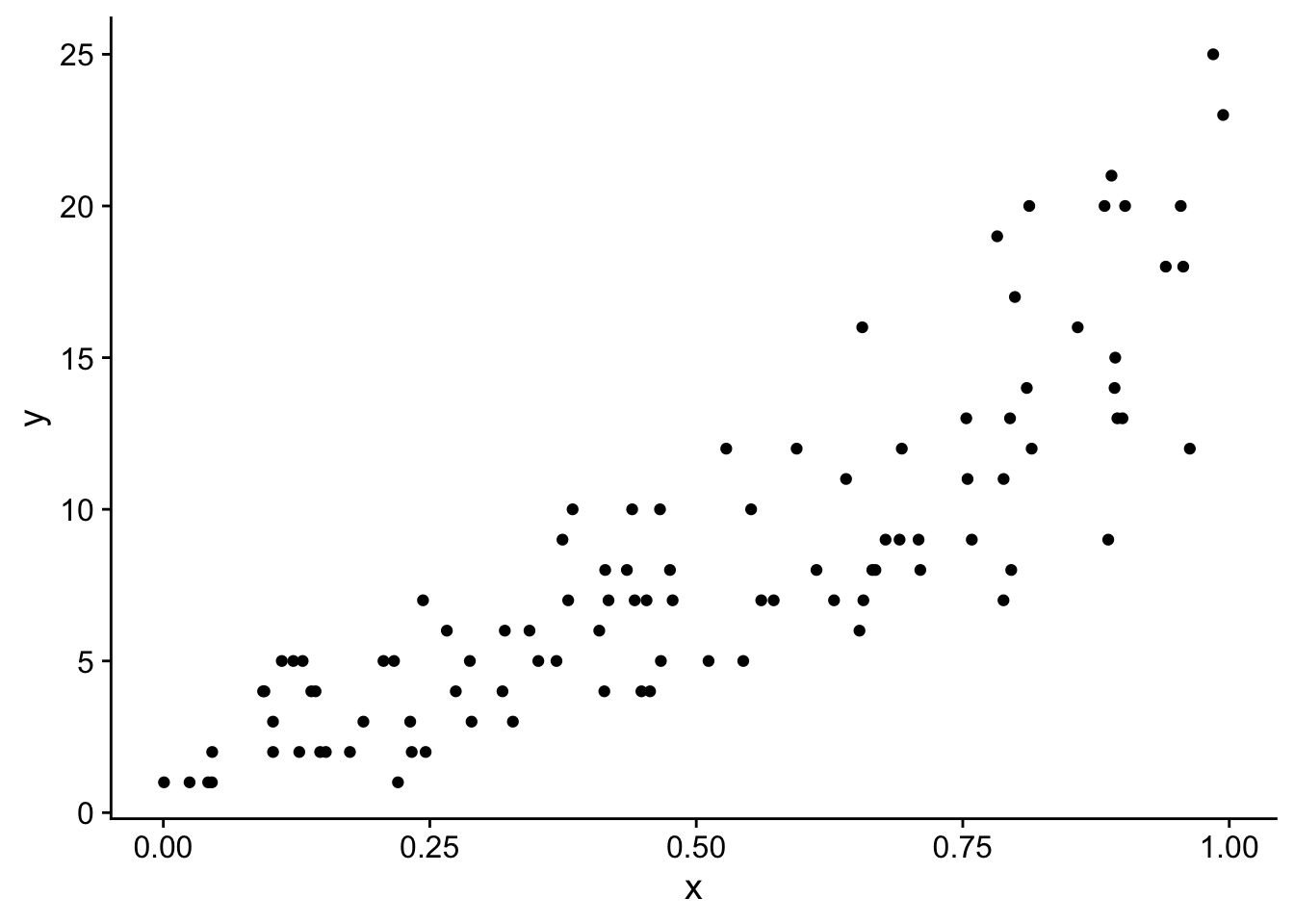
Now we can build a model of y as it responds to x:
mod <- glm(y ~ x, family = poisson)1.2 What is a model?
Let’s have a look at what R tells us about this model we just made:
mod
Call:  glm(formula = y ~ x, family = poisson)

Coefficients:
(Intercept)            x
     0.8888       2.1178

Degrees of Freedom: 99 Total (i.e. Null);  98 Residual
Null Deviance:      353.5
Residual Deviance: 79.36    AIC: 457.7
We see there are estimated coefficients: (Intercept) and x. The intercept is just that, the intercept, and the x coefficient is actually the slope. But what intercept and what slope? These words imply an equation, and in fact the equation was hiding in the code we used to simulate data. We said
# calculate the mean of `y` as a function of `x`
lambda <- exp(1 + 2 * x)

# finally calculate `y`
y <- rpois(length(x), lambda)
The equation hiding in this code is
\[\begin{align} y &\sim Pois(\lambda) \text{, where} \\ \lambda &= \exp(b_0 + b_1 x) \end{align}\]
This says that \(y\) is distributed according to a Poisson distribution (because we’re doing Poisson GLM) and that the mean of this Poisson distribution is a function of \(x\). Specifically, that function of \(x\) is \(\lambda = \exp(b_0 + b_1 x)\). So the slope is \(b_1\) and the intercept is \(b_0\). If we log transformed both sides we can more clearly see how \(b_0\) is the intercept and \(b_1\) the slope:
\[\begin{align} &\log(\lambda) = \log(\exp(b_0 + b_1 x)) \\ \Rightarrow &\log(\lambda) = b_0 + b_1 x \end{align}\]
That we take the log of \(\lambda\) is consistent with the fact that the Poisson GLM uses a log “link function” by default.
In our simulated data we set \(b_0 = 1\) and \(b_1 = 2\). Looking back at the output of the glm function we can see that our estimates are very close to those values!
mod
Call:  glm(formula = y ~ x, family = poisson)

Coefficients:
(Intercept)            x
     0.8888       2.1178

Degrees of Freedom: 99 Total (i.e. Null);  98 Residual
Null Deviance:      353.5
Residual Deviance: 79.36    AIC: 457.7
We can directly access those estimates like this:
b0_est <- mod$coefficients[1]
b1_est <- mod$coefficients[2]

b0_est
(Intercept)
0.8887906 b1_est x
2.117753 But how are those estimates actually made? That’s the job for likelihood.
1.3 What is a likelihood?
tl;dr: likelihood is the probability of the data given the model and its parameters. The parameter estimates for our model are exactly the parameter values that produce the maximum possible likelihood of the data. We call them the maximum likelihood estimates.
What does that mean? Let’s start with “probability of the data given the model and its parameters”. Remember from our equations, we are modeling \(y\) as coming from a Poisson distribution with mean \(\lambda\), \(\lambda\) is itself a function of \(x\) with parameters \(b_0\) and \(b_1\). So if we want to know the probability of any given data point (we’ll call any given data point \(y_i\)) then we just need to ask for the probability from the Poisson distribution, like this:
i <- 6 # let's look at the 6th data point
y_i <- dat$y[i]

# calculate lambda for data point i
lambda_i <- exp(b0_est + b1_est * dat$x[i])

dpois(y_i, lambda = lambda_i)
[1] 0.1839187That’s the probability of one data point, what about the probability of the entire dataset? Recall that probabilities multiply for independent observations, so the probability of the entire dataset is
\[\begin{align} P(Y) &= P(y_1) \times P(y_2) \times P(y_2) \times \cdots \times P(y_n) \\ \Rightarrow P(Y) &= \prod_{i = 1}^n P(y_i) \end{align}\]
This probability \(P(Y)\) is exactly the likelihood. We might write it as
\[ \mathcal{L}(Y | b_0, b_1) = \prod_{i = 1}^n P(y_i | b_0, b_1) \]
We added the “\(| b_0, b_1\)” to emphasize that the probability and likelihood depend on the values of \(b_0\) and \(b_1\).
In R code we can calculate that math like this:
allProbs <- dpois(y, exp(b0_est + b1_est * x))
prod(allProbs)
[1] 3.08673e-99Shoot! The probability is \(3.0867301\times 10^{-99}\), so….basically 0. This is why when working with likelihoods we actually use the log likelihood. Taking the log of a product (i.e. multiplication) turns it into summation. We typically use a little \(\mathcal{l}\) for log likelihood. So our math becomes
\[\begin{align} &\log(\mathcal{L}(Y | b_0, b_1)) = \log\left( \prod_{i = 1}^n P(y_i | b_0, b_1) \right) \\ \Rightarrow &\mathcal{l}(Y | b_0, b_1) = \sum_{i = 1}^n \log\left( P(y_i | b_0, b_1) \right) \end{align}\]
And our code becomes
allLogProbs <- dpois(y, exp(b0_est + b1_est * x), log = TRUE)
sum(allLogProbs)
[1] -226.8288Sweet! Our log likelihood is negative (no problem) and a reasonable number, not something basically equal to 0.
How does this help us find our parameter estimates? To find out, let’s calculate the log likelihood of our data, but with a different value for the slope, say \(b_1 = -1\).
l_neg1 <- dpois(y, exp(b0_est - 1 * x), log = TRUE)
sum(l_neg1)
[1] -1259.075That’s a much more negative log likelihood!
Let’s try another value, say \(b_1 = 4\)
l_pos4 <- dpois(y, exp(b0_est + 4 * x), log = TRUE)
sum(l_pos4)
[1] -1556.177That is also a much more negative number compared to the log likelihood at the actual estimated slope that R gave us. If we made a graph of how the log likelihood changes across different possible values of \(b_1\) it would look like this:
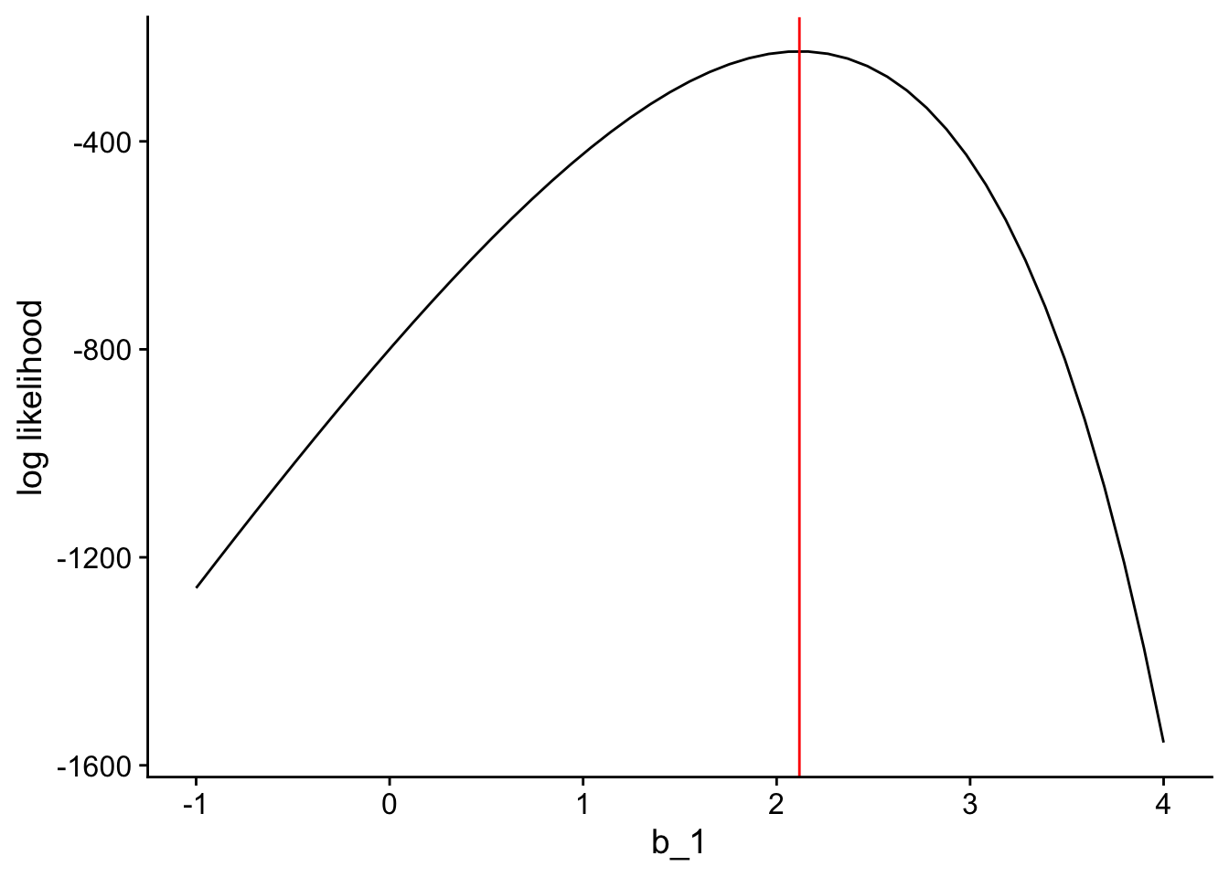
The log likelihood reaches its maximum value at exactly the value of \(b_1\) which the glm function gives us (shown in red).
So the parameter estimates that maximize the log likelihood of the data are the best possible parameter estimates for our model! And that’s how likelihood allows us to estimate parameters.
1.4 Akaike Information Criterion
So we can use log likelihood to estimate parameters, anything else? Yes! For one thing we can use log likelihood to help us decide between competing models. Competing models is the scenario where you have more than one possible model that you think could predict the data at hand and you want to decide which one does the best job relative to all the others.
In our simple example where we have y as some kind of count data and x as an explanatory variable, competing models could mean, for example, we have another explanatory variable w and we want to know which variable(s) do(es) the best job at predicting y.
Let’s make this concrete with code and some more simulated data
# simulate w as random numbers that in fact have nothing to do with y
w <- runif(length(x))

# add w to our data.frame
dat$w <- w

# visualize y versus x and y versus w
px <- ggplot(dat, aes(x = x, y = y)) +
    geom_point() +
    theme_cowplot()

pw <- ggplot(dat, aes(x = w, y = y)) +
    geom_point() +
    theme_cowplot()

plot_grid(px, pw, nrow = 1)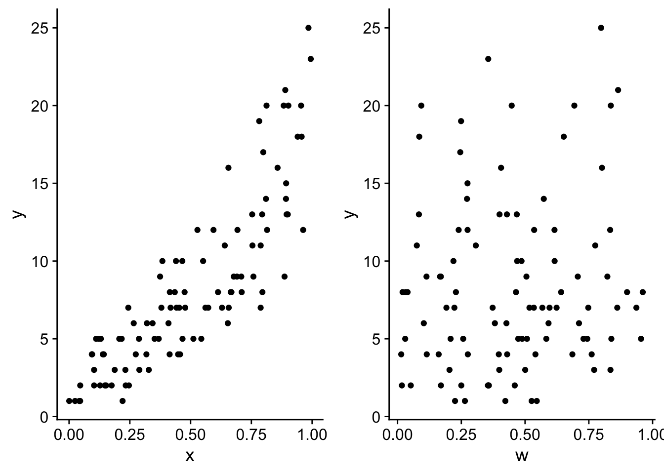
As we intended there is no real trend in y across w. But let’s compare the likelihoods of the model with only x and a model with x and w:
mod_with_w <- glm(y ~ x + w, family = poisson)


logLik(mod_with_w)
'log Lik.' -226.8016 (df=3)logLik(mod)'log Lik.' -226.8288 (df=2)The likelihood of the model with w is actually slightly higher (i.e. less negative) than the model with only x. He aha lā?! It turns out that adding more parameters to a model (even if they’re attached to nonsense explanatory variables) will always improve the likelihood of the data given the model. This is because every added parameter allows the model to capture a little more of the noise in the data, thus increasing the probability of the data given the model—that is, improving the likelihood. But we actually don’t want to fit our model to the noise, we want to fit our model to the real biology of what’s going on in the data.
So how can we decide which model is best when simply adding nonsense paramters will always improve the likelihood? This is the job of Akaike Information Criterion or “AIC”. AIC is a metric that describes how much a model is supported by the data. It is directly related to the log likelihood, but it penalizes models for the number of parameters they include, the more parameters, the higher the penalization. The equation for AIC is
\[ AIC = 2k - 2l \] where \(k\) is the number of fitted parameters in the model and \(l\) is the log likelihood. Let’s look at the AIC values for our two models
AIC(mod_with_w)[1] 459.6033AIC(mod)[1] 457.6576A smaller AIC indicates better model support, and sure enough the AIC of the model with only x is smaller by about 2 points.
AIC is helpful for telling us which model is relatively more supported by the data, but it does not tell us at all if the best supported model is actually any good. Just that it’s better than the other options. To figure out if the model is actually any good at predicting the data, we need a different approach.
1.5 Likelihood ratio test
Enter the likelihood ratio test—this can actually give us some insight as to whether our model is any good at predicting the data. We often abbreviate the likelihood ratio test as LRT, we’ll adopt that starting now.
In the case of our preferred model of y as a function of x, to know if this model is any good, we need to figure out if knowing x actually helps us predict the values of y. Put another way, is modeling y as a function of x any more predictive than a model with only an intercept (i.e. a flat line through the mean of y)? The LRT answers that question for us through a null hypothesis test that produces a \(p\)-value. The null hypothesis is that the likelihood for the flat line model with only intercept is statistically indistinguishable from the likelihood for the full model, the over with intercept and a slope for x.
We often call the model with fewer parameters, in this case the over with just the intercept, the “reduced model”. Let’s indicate the full model with all its parameters as \(m\) and the reduced model as \(m_0\). Then our two log likelihoods are
\[\begin{align} \mathcal{l}_0 &= \log \mathcal{L}(y | m_0) \\ \mathcal{l} &= \log \mathcal{L}(y | m) \end{align}\]
And the test statistic for the LRT is
\[ LRT = -2 (\mathcal{l}_0 - \mathcal{l}) \]
You might be wondering, where is the ratio (aka fraction) in this test statistic? Recall that logarithms have some special rules so that
\[ -2 (\mathcal{l}_0 - \mathcal{l}) = \log\left( \frac{\mathcal{L}(y | m_0)}{\mathcal{L}(y | m)} \right) \]
So the LRT test statistic is \(-2\) times the log of the ratio of the reduced model likelihood over the full model likelihood.
It turns out that under the null hypothesis—of indistinguishable likelihoods—this test statistic has a \(\chi^2\) distribution with degrees of freedom equal to the difference in the number of fitted parameters between the models. The reduced model has one fitted parameter, the intercept, and the full model has two, intercept and slope. So the degrees of freedom for the null \(\chi^2\) distribution.
Let’s calculate the \(LRT\) test statistic for our analysis and then calculate the \(P\)-value from the test statistic and relevant \(\chi^2\) distribution
# first we need to make the reduced model
# the formula `y ~ 1` is how we tell R to just estimate the intercept, no slopes
mod_0 <- glm(y ~ 1, data = dat, family = poisson)

# now we can calculate lrt = -2 * (l_0 - l)
lrt <- -2 * (logLik(mod_0) - logLik(mod))

# finally let's calculate the p-value by seeing where this test statistic
# falls with repsect to the upper tail of the chi^2 distribution
pchisq(lrt, df = 1, lower.tail = FALSE)
'log Lik.' 1.409661e-61 (df=1)So the \(P\)-value is \(1.4096614\times 10^{-61}\), which is basically 0, and indeed that is less than our typical \(\alpha = 0.05\) cutoff for statistical significance. So we reject the null hypothesis of indistinguishable likelihoods and conclude that the model including a slope for x indeed does a better job predicting the data.
1.6 Key differences between AIC and LRT
One key difference we already know is that AIC does not tell us if the model is a good fit to the data, it only helps us choose the best model out of two or more models that we are considering. All the models could in fact be bad and then AIC will just tell us which is the least bad. Conversely, the LRT can actually tell us if the model we’re interested in does a better job of predicting the data than a more simplified model. If our model of interest is better at prediction than a more simplified model, we have reason to conclude our model is actually relevant and meaningful.
Another key difference between AIC and LRT is when each approach is statistically appropriate and not appropriate. AIC can technically be used to compare any collection of models, while the LRT only works for “nested models.” What are nested models? They are any two models where the “simpler” model contains a subset of the parameters from the full model and no other parameters not contained in the full model. So the example we’ve been working with of \(m_0\) and \(m\) meets this criterion. We can see this clearly if we write the equations for each.
The full model is:
\[\begin{align} Y &\sim Pois(\lambda) \\ \lambda &= exp(b_0 + b_1 x) \end{align}\]
The reduced model is:
\[\begin{align} Y &\sim Pois(\lambda_0) \\ \lambda_0 &= exp(b_0) \end{align}\]
So the reduced model and full model both have parameter \(b_0\), but only the full model has parameter \(b_1\), this means the parameters of the reduced model are a subset of, are “nested within,” the parameters of the full model.