This lab will revisit simple linear models from a likelihood framework.
You can download the lab template .qmd file for this lab here:
The template will prompt you to work through the following sections.
14.1 The “simple” in simple linear models
The “simple” really just means we’re working with data that can be assumed to come from a normal distribution. Such a case is seen as simple largely for historical reasons—if the residuals of a regression (a kind of linear model) are normal, the by-hand calculations we used to have to do were simpler. “Simple” does not refer to the complexity of the question our model addresses or the number of explanatory variables.
In this lab we will look at the process of going from question to prediction to model for two questions:
Do native trees versus non-native trees have different average sizes (DBH’s)?
How does the human impact index influence tree size (DBH)?
Before we get started, let’s read in the data. We will need the tree data, but also the human impact index from hii_geo.csv file.
# still reading-in from githubtree <-read.csv("https://raw.githubusercontent.com/uhm-biostats/stat-mod/refs/heads/main/data/OpenNahele_Tree_Data.csv")hii_geo <-read.csv("https://raw.githubusercontent.com/uhm-biostats/stat-mod/refs/heads/main/data/hii_geo.csv")# merge the data into one data.framedat <-left_join(tree, hii_geo)
Joining with `by = join_by(PlotID)`
While we’re on the topic of data, let’s clean it up a little
dat <- dat |># remove missing DBH valuesfilter(!is.na(DBH_cm)) |># add a column for log-transformed DBH since this will be # the variable we use as a response variablemutate(log_dbh_cm =log(DBH_cm)) |># remove NAs for elevationfilter(!is.na(hii)) |># remove "uncertain" for native statusfilter(Native_Status !="uncertain")
We could go much further in cleaning-up the data.frame, but for our purposes we will be fine to leave it as is.
14.2 DBH of native versus non-native trees
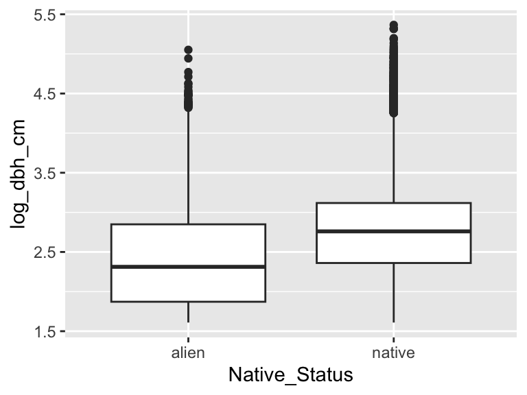
To go from question to model, we need to pass through prediction. For the question of “do native trees versus non-native trees have different average DBH?” what is our prediction? We might look around at the huge Albizia trees all around and think that non-native trees tend to be larger. We could make a conceptual graphic to visualize this prediction, but we have the data in hand, so let’s go ahead and look at the real data. But one note of caution: looking at the data too much can lead us down the route of “data dredging”—where we sift through the data looking for something “significant” looking. With that caution in mind, we have our question and prediction, and we will just focus on that:
The data show the opposite pattern from our prediction. Interesting! But ultimately no matter, we have successfully identified the variables we need for our model: Native_Status and log_dbh_cm.
Now we need to think about the source of variability. We have previously discussed that log-transformed DBH has reason to be normally distributed thanks to the central limit theorem. We will go with that. How do we combine the variables with a normal distribution? Let’s think of how we would simulate.
# make a vector of "native" and "non-native", just a few will dox <-c("native", "native", "native", "non-native", "non-native", "non-native")# pick an average log DBH for native trees---this is a *parameter*mean_native <-2.75# pick an average log DBH for non-native trees---another *parameter*mean_nonnat <-2.25# make a vector for mean log DBH (for plugging into `rnorm`)m <-ifelse(x =="native", mean_native, mean_nonnat)# check out mm
[1] 2.75 2.75 2.75 2.25 2.25 2.25
# simulate log DBH with an SD of 1y <-rnorm(length(m), mean = m, sd =1)
Notice what we did there to make the mean. We used ifelse to make a vector where elements corresponding to x = "native" get the value of mean_native, and elements corresponding to x = "non-native" get the value of mean_nonnat.
So the mean of the normal distribution is a function of native-status and the standard deviation is just some value. We can use this simulation exercise to write our log-likelihood function. The parameters that we will search over to find a maximum are \(\mu_\text{native}\), \(\mu_\text{non-native}\), and \(\sigma\). The data we will use is composed of log_bdh_cm as the response variable and Native_Status as the explanatory variable.
# let's let `x` be explanatory and `y` be response variablesloglik_nat <-function(pars, explan_var, respon_var) {# browser()# extract parameters mu_nat <- pars[1] mu_non <- pars[2] sig <- pars[3]# create vector of means mu <-ifelse(explan_var =="native", mu_nat, mu_non)# compute log likelihooddnorm(respon_var, mean = mu, sd = sig, log =TRUE) |>sum()}
We should note we have also now seen a longer function than the one or two line examples we had written in previous labs.
Now it’s up to you to find the maximum with optim.
14.3 How does the human impact index influence DBH?
you can delete these prompts once complete, or turn them into subheadings
Now you’re on your own, but you got this! Walk through these same steps but for the question of the relationship between human impact index and log DBH. For ease of finding it, the human impact index is stored in the column hii in our dat data object. The steps are:
Produce a prediction from the question
Use a data visualization to help you understand that prediction and identify response and explanatory variables
Identify the source of variance you will model; thinking about how you might simulate similar data can help
Write the log likelihood function; if you thought through data simulation, this can help here as well