17 Working with mixed effects models in R

This lab will walk us through how to use the lme4 package to fit a mixed effects model.

You can download the lab template .qmd file for this lab here:

The template will prompt you to work through the following sections.

17.1 Using simulated data to understand fitting mixed effects models

Let’s start with some simulated data to both make sure we understand how mixed effects model work (and their assumptions) and how the lme4 package implements fitting mixed effects models.

First we simulate the data. Imagine we have some response variable y and some numeric explanatory variable x and we have collected data on these variables from 8 sites (think sampling locations across space) with 20 observations coming from each site.

# set-up the simulation

# number of sites (will be rand effect)
nsite <- 8

# number of (pseudo) reps per site
nrep <- 20

# sd of the random effect of site
sig_rand <- 1

# sd of the "residuals"
sig_resid <- 0.25

# overall intercept
a0 <- 8

# slope
a1 <- 2

sim_dat <- data.frame(site = rep(paste0("site_", 1:nsite), each = nrep), 
                      # simulate random effect of site, we would never
                      # actually have this in real data
                      site_rand = rep(rnorm(nsite, mean = 0, sd = sig_rand), 
                                      each = nrep),
                      x = runif(nsite * nrep)) |> 
    # add the response variable
    mutate(y = rnorm(nsite * nrep, 
                     mean = a0 + site_rand + a1 * x, 
                     sd = sig_resid))

head(sim_dat)

    site site_rand          x         y
1 site_1  1.697885 0.77202315 11.033307
2 site_1  1.697885 0.21750979 10.162655
3 site_1  1.697885 0.68475055 10.711050
4 site_1  1.697885 0.09434311  9.770182
5 site_1  1.697885 0.87380343 11.510986
6 site_1  1.697885 0.30712589  9.996297

Let’s have a look at these data

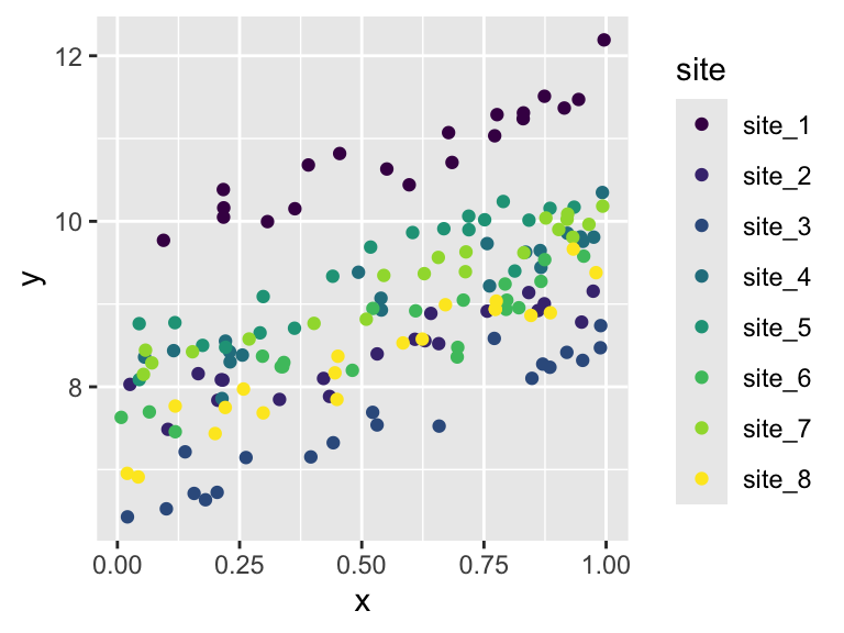
ggplot(sim_dat, aes(x, y, color = site)) +
    geom_point() +
    scale_color_viridis_d()

We can see that the random effect of site bumps the observations up or down but does not change the slope of y versus x. So the rand effect of site only impacts the intercept (more on that shortly).

This is indeed what we should expect because this is how we simulated the data, we said the mean of y is

a0 + site_rand + a1 * x

The site_rand enters this expression as an additional intercept term along with a0.

17.1.1 Introducing lme4 and the `lmer` function

Now we are going to try to use maximum likelihood to estimate the values of the parameters a0, a1, sig_rand, and sig_resid from the simulated data. We know the “true” values of those parameters, so we can evaluate whether the maximum likelihood method implemented in lmer worked.

Here is how to use the lmer function:

sim_mod <- lmer(y ~ x + (1 | site), data = sim_dat, REML = FALSE)

Notice a few things:

The fixed effects part of the model is like what we’ve seen before: y ~ x
The way a random effect is implemented is through the notation (1 | site) which means “let there be an additional intercept term conditional on site”
We also had to specify REML = FALSE, this is because the default is REML = TRUE and that default actually does not maximize the likelihood function (what we want) but rather maximizes the “relative” or “residual” likelihood (what we don’t want)

Now we can look at the results

sim_mod

Linear mixed model fit by maximum likelihood  ['lmerMod']
Formula: y ~ x + (1 | site)
   Data: sim_dat
      AIC       BIC    logLik -2*log(L)  df.resid 
  43.1723   55.4730  -17.5862   35.1723       156 
Random effects:
 Groups   Name        Std.Dev.
 site     (Intercept) 0.8655  
 Residual             0.2347  
Number of obs: 160, groups:  site, 8
Fixed Effects:
(Intercept)            x  
      7.835        2.022

The print-out should show us a standard deviation for random effect site that is close to 1 and a standard deviation for the residuals that is close to 0.25. If we want to directly access those values we can like this:

# extract the fixed effects
fixef(sim_mod)

(Intercept)           x 
   7.834852    2.022116

# extract the standard deviations of random effects
VarCorr(sim_mod)

 Groups   Name        Std.Dev.
 site     (Intercept) 0.86551 
 Residual             0.23475

Something interesting about the way mixed effects models are fit is that the algorithm actually infers the optimal values that should be sampled from the random effect to maximize the likelihood. We can see evidence of that by asking for the “coefficients” of the model

coef(sim_mod)

$site
       (Intercept)        x
site_1    9.623717 2.022116
site_2    7.364343 2.022116
site_3    6.497422 2.022116
site_4    7.957060 2.022116
site_5    8.353393 2.022116
site_6    7.499828 2.022116
site_7    8.093754 2.022116
site_8    7.289295 2.022116

attr(,"class")
[1] "coef.mer"

We see an intercept for each site. The fact that each site gets its own (randomly sampled) intercept is why this kind mixed effects model is call a “random intercepts” model.

17.2 Fitting a mixed effects model to real data

Now its your turn to take what we learned with simulated data and fit a random intercepts model to the real data. Let’s return to the model of trying to predict log DBH based on human impact and invasive status (with an interaction) but now we’ll include a random effect of survey plot. The fixed effects part of the model should be the same as before and look like this:

log_dbh_cm ~ Native_Status * hii

First load and clean the data as we have before:

tree <- read.csv("https://raw.githubusercontent.com/uhm-biostats/stat-mod/refs/heads/main/data/OpenNahele_Tree_Data.csv")

hii_geo <- read.csv("https://raw.githubusercontent.com/uhm-biostats/stat-mod/refs/heads/main/data/hii_geo.csv")

# merge the data into one data.frame, clean, add needed columns
dat <- left_join(tree, hii_geo) |> 
    # remove missing DBH values
    filter(!is.na(DBH_cm)) |> 
    # add a column for log-transformed DBH since this will be 
    # the variable we use as a response variable
    mutate(log_dbh_cm = log(DBH_cm)) |> 
    # remove NAs for elevation
    filter(!is.na(hii)) |> 
    # remove "uncertain" for native status
    filter(Native_Status != "uncertain")

Joining with `by = join_by(PlotID)`

Now take it from there!

17.1 Using simulated data to understand fitting mixed effects models

17.1.1 Introducing lme4 and the lmer function

17.2 Fitting a mixed effects model to real data

17.1.1 Introducing lme4 and the `lmer` function